Jones-matrix imaging of biological tissues with quadruple-channel optical coherence tomography

Shuliang Jiao; Lihong V. Wang

doi:10.1117/1.1483878

1 July 2002 Jones-matrix imaging of biological tissues with quadruple-channel optical coherence tomography

Shuliang Jiao, Lihong V. Wang

Author Affiliations +

Journal of Biomedical Optics, Vol. 7, Issue 3, (July 2002). https://doi.org/10.1117/1.1483878

1. Introduction

As a result of its noninvasive characteristic, its high spatial resolution, and its easy optical fiber implementation, optical coherence tomography (OCT) is emerging as an important optical imaging modality. Various technical approaches have been developed to increase the spatial resolution,¹ ² imaging rate,³ ⁴ and image quality.⁵ ⁶ To completely retrieve information on the backscattered light field, both amplitude and polarization information need to be recorded. Conventional OCT systems record only the amplitude but not information on the polarization of scattered light. In contrast, polarization-sensitive OCT can capture the polarization states of backscattered light and as a result can reveal the polarization properties, such as birefringence, of a sample which are not available in conventional OCT.⁷ ⁸ ⁹ ¹⁰ ¹¹ ¹² Birefringence is related to various biological components such as collagen, muscle fibers, myelin, retina, keratin, and glucose. Consequently, polarization can provide novel contrast mechanisms for imaging, diagnosis, and sensing. In Mueller calculus, the polarization state of light can be completely characterized by a Stokes vector and the polarization transforming properties of an optical sample can be completely characterized by a Mueller matrix. A combination of Mueller calculus and OCT offers a unique way by which to acquire the Mueller matrix of a scattering sample with OCT resolution.¹⁰ ¹¹ Yao and Wang¹⁰ first reported two-dimensional depth-resolved Mueller-matrix images of biological tissues measured with OCT based on 16 combinations of source and analyzing polarization states. The relatively time-consuming nature of the measurement process limited the application of the technique to stable samples such as bones. Jiao et al.;¹¹ further demonstrated that the degree of polarization (DOP) of the backscattered light measured by OCT is unity throughout the range of detection, where a DOP of unity indicates that the measured Mueller matrix is nondepolarizing. This conclusion allows the use of a Jones matrix instead of a Mueller matrix in OCT.

To measure less stable samples such as soft tissues, we recently developed a system that can determine the Jones matrix with a single depth scan (A scan). In other words, this system can acquire the Jones matrix as fast as its conventional OCT counterpart can acquire a regular image. The measured Jones matrix can be further transformed into an equivalent Mueller matrix if desired.¹² Several types of biological tissues were tested with this system and the images of the Jones matrices were analyzed.

2. Jones Matrix and Mueller Matrix

A Jones matrix (J) transforms an input Jones vector (E _in) into an output Jones vector (E _out) while a Mueller matrix (M) transforms an input Stokes vector (S _in) into an output Stokes vector (S _out):

Eq. (1)

E_{out} = [\begin{matrix} E_{OH} \\ E_{OV} \end{matrix}] = {JE}_{in} = [\begin{matrix} J_{11} & J_{12} \\ J_{21} & J_{22} \end{matrix}] [\begin{matrix} E_{iH} \\ E_{iV} \end{matrix}],

Eq. (2)

S_{out} = [\begin{matrix} S_{0} \\ S_{1} \\ S_{2} \\ S_{3} \end{matrix}] = {MS}_{in} = [\begin{matrix} M_{00} & M_{01} & M_{02} & M_{03} \\ M_{10} & M_{11} & M_{12} & M_{13} \\ M_{20} & M_{21} & M_{22} & M_{23} \\ M_{30} & M_{31} & M_{32} & M_{33} \end{matrix}] [\begin{matrix} S_{i 0} \\ S_{i 1} \\ S_{i 2} \\ S_{i 3} \end{matrix}],

where E_OH and E_OV are the horizontal and vertical components of the electric vector of the output light field; E_iH and E_iV are the horizontal and vertical components of the electric vector of the input light field; S₀, S₁, S₂, and S₃ are the elements of the Stokes vector of the output light; and S_i0, S_i1, S_i2, and S_i3 are the elements of the Stokes vector of the input light, respectively. S₀ and S_i0 are the intensity of the output and input light, respectively. In an OCT system, S_i0 represents the intensity of the incident light in the sample arm, and S₀ represents the detected intensity of the backscattered light. In Eq. (2), we can clearly see that M₀₀ represents the intensity transformation property of the sample and contains no polarization information. The degree of polarization of the output light is defined as

Eq. (3)

DOP = \frac{\sqrt{S_{1}^{2} + S_{2}^{2} + S_{3}^{2}}}{S_{0}} .

The degree of polarization of the input light can also be defined in the same way as the DOP of the output light with the input Stokes vector. If the DOP of a light field remains unity after transformation by an optical system, the system is nondepolarizing; otherwise, the system is depolarizing.

The Jones matrices of a homogeneous partial polarizer (J _P) and a homogeneous elliptical retarder (J _R) can be expressed as

J_{P} = [\begin{matrix} P_{1} {cos}^{2} α + P_{2} {sin}^{2} α & (P_{1} - P_{2}) sin α cos α e^{- i Δ} \\ (P_{1} - P_{2}) sin α cos α e^{i Δ} & P_{1} {sin}^{2} α + P_{2} {cos}^{2} α \end{matrix}],

J_{R} = [\begin{matrix} e^{i φ / 2} {cos}^{2} θ + e^{- i φ / 2} {sin}^{2} θ & (e^{i φ / 2} - e^{- i φ / 2}) sin θ cos θ e^{- i δ} \\ (e^{i φ / 2} - e^{- i φ / 2}) sin θ cos θ e^{i δ} & e^{i φ / 2} {sin}^{2} θ + e^{- i φ / 2} {cos}^{2} θ \end{matrix}],

where P₁ and P₂ are the principal coefficients of the amplitude transmission for the two orthogonal polarization eigenstates; α is the orientation of J _P; φ and θ are the retardation and orientation of J _R; Δ and δ are the phase differences of the vertical and horizontal components of the eigenstates of J _P and J _R, respectively. A retarder is called elliptical when its eigenvectors are those of elliptical polarization states. A polarizing element is called homogeneous when the two eigenvectors of its Jones matrix are orthogonal.¹³ ¹⁴ Linear polarizers and linear and circular retarders are typical homogeneous polarizing optical elements. A typical example of inhomogeneous polarizing elements is the circular polarizer, whose Jones matrix is

\frac{1}{2} [\begin{matrix} 1 & 1 \\ i & i \end{matrix}],

which is constructed by using a linear polarizer set at 45° followed by a quarter-wave plate (λ/4 plate) with its fast axis set horizontal. The eigenvectors of such a circular polarizer are

\frac{1}{\sqrt{2}} [\begin{matrix} 1 \\ - 1 \end{matrix}]

for a −45° linear polarization state and

\frac{1}{\sqrt{2}} [\begin{matrix} 1 \\ i \end{matrix}]

for a right circular polarization state, which are not orthogonal.

For an intensity-based noninterference detection system, a turbid medium is generally depolarizing unless the detector is small; in other words, when a completely polarized light (DOP=1) is scattered by the medium, the output light becomes partially polarized (DOP<1) unless the area of detection is much less than the average size of speckles.¹⁵ However, OCT is an amplitude-based detection system that uses interference heterodyne, which detects the part of the backscattered electric field that is coherent with the reference beam, regardless of whether the backscattered light is partially polarized or not. The OCT signal I_OCT received by a detector of finite area can be considered the sum of contributions from the backscattered optical fields E _si that reach various points of the detector:

Eq. (4)

\begin{matrix} I_{OCT} & = & E_{r} \cdot E_{s 1} + E_{r} \cdot E_{s 2} + E_{r} \cdot E_{s 3} + \dots \\ = & E_{r} \cdot (E_{s 1} + E_{S 2} + E_{s 3} + \dots) \\ = & E_{r} \cdot E_{s} . \end{matrix}

where E _r represents the reference optical field; E _s is an equivalent backscattered optical field; and the dot product represents the interference signal (apart from a constant factor). As shown in Eq. (4), each backscattered optical field from the sample contributes to the OCT signal by projecting onto the reference optical field E _r. Equivalently, the backscattered optical fields that reach various points of the detector can be summed in vector, and the vector sum E _s is then projected onto the reference optical field to yield the OCT signal. One can imagine this as being equivalent to shrinking the full field over the area of detection to a single point before interfering with the reference beam. If all of the E _si share the same polarization state, E _s will have the same polarization state; otherwise, E _s will have a net apparent polarization state. In either case, the E _s measured will have a unique polarization state. As a result, the DOP measured by OCT will be unity. In an intensity-based noninterference detection system, in contrast, the backscattered optical fields that reach various points of the detector would add in intensity. In that case, if all the E _si do not share the same polarization state, the DOP will be less than unity.

Unlike a Mueller matrix, which is suited to all kinds of optical systems, a Jones matrix can only be applied to a nondepolarizing optical system. A Jones matrix can completely characterize the polarization properties of a nondepolarizing optical system. In other words, for a nondepolarizing optical system, a Jones matrix is equivalent to a Mueller matrix. A Jones matrix has four complex elements, in which one phase is arbitrary and consequently seven real parameters are independent. Equivalently, there are seven independent parameters in a nondepolarizing Mueller matrix.

When the two matrices are equivalent, one matrix is preferred over the other in some situations. A Jones matrix has fewer elements and the physical meanings of the matrix elements are clearer. On the other hand, a Mueller matrix uses only real numbers, and the intensity transformation property of a sample is explicitly expressed in its M₀₀ element, which provides an image of the sample without the influence of its polarization property. M₀₀ contains no polarization artifact like that usually encountered in a conventional OCT image when the sample contains birefringence. Therefore, a Mueller matrix clearly separates structural information from polarization information of a sample.

The Jones matrix of a nondepolarizing optical system can be transformed into an equivalent nondepolarizing Mueller matrix by the following relationship:¹⁶

Eq. (5a)

\begin{matrix} M & = & U (J \otimes J^{*}) U^{- 1}, \\ = & U [\begin{matrix} J_{11} J^{*} & J_{12} J^{*} \\ J_{21} J^{*} & J_{22} J^{*} \end{matrix}] U^{- 1} \\ = & U [\begin{matrix} J_{11} J_{11}^{*} & J_{11} J_{12}^{*} & J_{12} J_{11}^{*} & J_{12} J_{12}^{*} \\ J_{11} J_{21}^{*} & J_{11} J_{22}^{*} & J_{12} J_{21}^{*} & J_{12} J_{22}^{*} \\ J_{21} J_{11}^{*} & J_{21} J_{12}^{*} & J_{22} J_{11}^{*} & J_{22} J_{12}^{*} \\ J_{21} J_{21}^{*} & J_{21} J_{22}^{*} & J_{22} J_{21}^{*} & J_{22} J_{22}^{*} \end{matrix}] U^{- 1}, \end{matrix}

and a Jones vector of a light field can be transformed into a Stokes vector by

Eq. (5b)

\begin{matrix} S & = & \sqrt{2} U (E \otimes E^{*}) = \sqrt{2} U [\begin{matrix} E_{H} E^{*} \\ E_{V} E^{*} \end{matrix}] \\ = & \sqrt{2} U [\begin{matrix} E_{H} E_{H}^{*} \\ E_{H} E_{V}^{*} \\ E_{V} E_{H}^{*} \\ E_{V} E_{V}^{*} \end{matrix}], \end{matrix}

where ⊗ represents the Kronecker tensor product and U is the 4×4 Jones–Mueller transformation matrix:

U = \frac{1}{\sqrt{2}} [\begin{matrix} 1 & 0 & 0 & 1 \\ 1 & 0 & 0 & - 1 \\ 0 & 1 & 1 & 0 \\ 0 & i & - i & 0 \end{matrix}] .

At least two independent incident polarization states, which are not necessarily orthogonal, are needed to fully determine a Jones matrix.

3. Experimental System

A schematic of the experimental setup is shown in Figure 1. Two superluminescent diodes (SLDs) are employed as low-coherence light sources and are amplitude modulated at 3 and 3.5 kHz by modulating the injection current. The two light sources are in horizontal and vertical polarization states, respectively, and each delivers about 200 μW of power to the sample. The center wavelength, full width at half maximum (FWHM) bandwidth, and the output power of the light sources are 850 nm, 26 nm, and 3 mW, respectively. The Jones vectors of the two sources are [1,0]^T and [0,1]^T, respectively, where the superscript T transposes the row vectors into column vectors. The two source beams are merged by a polarizing beam splitter (PBS1), filtered by a spatial filter assembly and then split into the reference arm and the sample arm by a nonpolarizing beam splitter (NBS). The sample beam passes through a λ/4 plate, the fast axis of which is oriented at 45° and is focused into the sample by an objective lens [L1: f=15 mm and numerical aperture (NA)=0.25 ]. The Jones vectors of the sample beam at the sample surface for the two sources are [1,i]^T and [1,−i]^T, which are right circularly and left circularly polarized, respectively. The reference arm consists of a λ/4 plate, the fast axis of which is oriented 22.5°, a lens (L2), and a mirror. After retroreflection by the reference mirror and double passing through the λ/4 plate, the horizontal polarization (H) of the incident light is converted into 45° polarization, [1,1]^T, while the vertical polarization (V) of the incident light is converted into −45° polarization, [1,−1]^T, and then the reference beam combines with the backscattered sample beam through the NBS. The combined light is split into two orthogonal polarization components, i.e., the horizontal and vertical components of the Jones vector, by a polarization beam splitter (PBS2). The two components are coupled into two single-mode fibers with objective lenses. The two polarization components are detected by photodiodes PDH and PDV, respectively. A data-acquisition board (DAQ board) sampling at 50 kHz/channel digitizes the two signals. The scan speed of the reference arm is 0.5 mm/s, generating a Doppler frequency of about 1.2 kHz. The carrier frequencies, 1.8, 2.3, 4.2, and 4.7 kHz, are the beat and harmonic frequencies between this Doppler frequency and the modulation frequencies of the light sources.

Figure 1

Schematic of the double-beam polarization-sensitive OCT system: SLDH and SLDV, superluminescent diodes, horizontally polarized (H) and vertically polarized (V), respectively; PBS1 and PBS2, polarizing beam splitters; SPF, spatial filter assembly; NBS, nonpolarizing beam splitter; QW1 and QW2, zero-order quarter-wave plates; M, mirror; L1, L2 L3 and L4, lenses; PDH and PDV, photodiodes for H and V polarization components.

The two function generators (DS345, Stanford Research Systems), which are used for modulation of the two light sources, respectively, are synchronized and share the same time base. Burst mode was used to ensure that the initial phases of the two modulation signals are fixed for each A scan. The time delay between scanning of the two channels of the DAQ board is 10 μs. The phase difference between the two channels caused by this time delay for each beat and harmonic frequency was compensated for during signal processing.

For OCT signals based on single-backscattered photons, the incident Jones vector E _i to the sample arm is transformed into the detected Jones vector E _o by

Eq. (6)

\begin{matrix} E_{o} & = & J_{NBS} J_{QB} J_{SB} J_{M} J_{SI} J_{QI} E_{i} \\ = & J_{NBS} J_{QB} {JJ}_{QI} E_{i} = J_{T} E_{i}, \end{matrix}

where J _QI and J _QB are the Jones matrices of the λ/4 plate for incident and backscattered light, respectively; J _SI and J _SB are the Jones matrices of the sample for incident and backscattered light, respectively; J _M is the Jones matrix of the single backscatterer, the same as the one for a mirror; J _NBS is the Jones matrix of the reflecting surface of the nonpolarizing beam splitter; J is the combined roundtrip Jones matrix of the scattering medium; J _T is the overall roundtrip Jones matrix.

In Eq. (6), the output Jones vector E _o is constructed for each light source from the measured horizontal and vertical components of the OCT signal. Upon acquiring the output Jones vectors and knowing the input Jones vectors, the overall roundtrip Jones matrix J _T can be calculated. The Jones matrix J of the sample can be extracted from J _T by eliminating the effect of the Jones matrices of the quarter-wave plate, the mirror, and the beam splitter. As a necessary condition, the two light sources must be independent of each other, which means that there is an arbitrary phase difference between the two measured Jones vectors for the two light sources. The arbitrary phase difference must be eliminated in order to calculate J _T.

In the commonly used convention, J _M transforms the polarization state of forward light expressed in the forward coordinate system into the polarization state expressed in the backward coordinate system. Similarly, J _NBS transforms the polarization state of backward light into the polarization state expressed in the detection coordinate system. However, in this work we express the polarization states of both forward and backward light in the forward coordinate system. With this convention, J _M and J _NBS are unitary:

J_{M} = J_{NBS} = [\begin{matrix} 1 & 0 \\ 0 & 1 \end{matrix}] .

In each A scan, the optical paths for forward and backward light are the same and, therefore, the Jones reversibility theorem can be applied.¹⁷ The Jones reversibility theorem indicates that the Jones matrices J _bwd and J _fwd of an ordinary optical element for backward and forward light propagation have the following relationship if the same coordinate system is used for the Jones vectors: J _bwd=J _fwd ^T. Therefore, we have the following relationships:

J_{SB} = J_{SI}^{T}, J_{QB} = J_{QI}^{T} = \frac{1}{\sqrt{2}} [\begin{matrix} 1 & i \\ i & 1 \end{matrix}],

J = J_{SB} J_{M} J_{SI} = J_{SI}^{T} J_{SI} = J^{T},

J_{T} = J_{NBS} J_{QB} {JJ}_{QI} = J_{QI}^{T} {JJ}_{QI} = J_{T}^{T} .

In other words, matrices J and J _T are transpose symmetric. This property of transpose symmetry is important for eliminating the arbitrary phase difference between the two light sources. Because of this symmetry, the number of independent parameters in the Jones matrix is further reduced from seven to five.

As reported by Yao and Wang using Monte Carlo simulation,¹⁸ light backscattered from the sample can be divided into two parts: class I and class II. Class I light provides a useful signal, which is scattered by the target layer in a sample and the pathlength difference of which from the reference light is within the coherence length of the light source. Class II light is the part scattered from the rest of the medium, whose pathlength difference from the reference light is also within the coherence length of the light source. Class II light contributes to background noise of the OCT signal. The weight of class II light in the detected OCT signal increases with depth and will exceed that of the class I signal beyond some critical depth. An increase in the weight of class II light deteriorates the resolution and signal-to-noise ratio and thus limits the effective imaging depth. The class I signal also contains multiply scattered photons, but due to the requirement of matching optical pathlengths, these multiple scattering events must be small-angle scattering.

For the multiply scattered photons, Eq. (6) still holds if the probability for photons to travel along the same roundtrip path but in opposite directions is equal, which is a valid assumption when the source and detector have reciprocal characteristics. Because these photons are coherent, the roundtrip Jones matrix of the sample J is the sum of the Jones matrices of all possible roundtrip paths; for each possible path, for example, the kth path, the roundtrip Jones matrix is the sum of the Jones matrices for the two opposite directions [ J _i(k) and J _r(k) ]. Consequently, we have

J = \sum_{k} [J_{i} (k) + J_{r} (k)] = \sum_{k} {J_{i} (k) + {[J_{i} (k)]}^{T}} = J^{T} .

In other words, J as well as J _T still possess transpose symmetry even if multiple scattering occurs as long as the source and the detector meet the condition.

After calculation, Eq. (6) can be expressed as

Eq. (7a)

\begin{matrix} [\begin{matrix} E_{o H} \\ E_{o V} \end{matrix}] & = & [\begin{matrix} \frac{i}{2} (J_{11} - 2 i J_{12} - J_{22}) & \frac{1}{2} (J_{11} + J_{22}) \\ \frac{1}{2} (J_{11} + J_{22}) & \frac{i}{2} (- J_{11} - 2 i J_{12} + J_{22}) \end{matrix}] \times [\begin{matrix} E_{i H} \\ E_{i V} \end{matrix}] \\ = & [\begin{matrix} J_{T 11} & J_{T 12} \\ J_{T 12} & J_{T 22} \end{matrix}] \times [\begin{matrix} E_{i H} \\ E_{i V} \end{matrix}], \end{matrix}

where J_ij and J_Tij (i,j=1,2) are the elements of J and J _T, respectively. For two light sources of independent polarization states, Eq. (7a) can be rearranged as

Eq. (7b)

[\begin{matrix} E_{oH 1} & E_{oH 2} \\ E_{oV 1} & E_{oV 2} \end{matrix}] = [\begin{matrix} J_{T 11} & J_{T 12} \\ J_{T 12} & J_{T 22} \end{matrix}] \times [\begin{matrix} E_{iH 1} & E_{iH 2} e^{i β} \\ E_{iV 1} & E_{iV 2} e^{i β} \end{matrix}],

where E_oH1 and E_oH2 and E_oV1 and E_oV2 are the elements of the Jones vectors of source 1 and source 2, respectively; β is the random initial phase difference between the two light sources due to their mutual independence. J _T can be calculated from Eq. (7b) as

Eq. (7c)

\begin{matrix} [\begin{matrix} J_{T 11} & J_{T 12} \\ J_{T 12} & J_{T 22} \end{matrix}] & = & [\begin{matrix} E_{o H 1} & E_{oH 2} \\ E_{oV 1} & E_{oV 2} \end{matrix}] \times {[\begin{matrix} E_{iH 1} & E_{iH 2} e^{i β} \\ E_{iV 1} & E_{iV 2} e^{i β} \end{matrix}]}^{- 1} \\ = & \frac{1}{D} [\begin{matrix} E_{oH 1} & E_{oH 2} \\ E_{oV 1} & E_{oV 2} \end{matrix}] \\ \times [\begin{matrix} E_{iV 2} e^{i β} & - E_{iH 2} e^{i β} \\ - E_{iV 1} & E_{iH 1} \end{matrix}], \end{matrix}

as long as the determinant,

D = | \begin{matrix} E_{iH 1} & E_{iH 2} e^{i β} \\ E_{iV 1} & E_{iV 2} e^{i β} \end{matrix} | = e^{i β} | \begin{matrix} E_{iH 1} & E_{iH 2} \\ E_{iV 1} & E_{iV 2} \end{matrix} | \neq 0,

i.e., the two light sources are not in the same polarization state. The random phase difference β can be eliminated with the transpose symmetry of J _T:

Eq. (7d)

e^{i β} (E_{oH 1} E_{iH 2} + E_{oV 1} E_{iV 2}) = (E_{oV 2} E_{iV 1} + E_{oH 2} E_{iH 1}) .

Equation (7d) can be solved when (E_oH1E_iH2+E_oV1E_iV2)≠0. Once J _T is found, J can then be determined from J _T. Six real parameters of J can be calculated, one phase of which is arbitrary and can be subtracted from each element, and eventually five independent parameters are retained.

When (E_oH1E_iH2+E_oV1E_iV2)=0, it is impossible to eliminate the random phase by using transpose symmetry. This situation happens if the sample arm does not alter the polarization states of the two incident beams besides producing a mirror reflection. For example, this situation occurs if (1) a horizontal or vertical incident beam is used, (2) a λ/4 plate is not inserted into the sample arm, and (3) the fast axis of a birefringent sample is horizontal or vertical. The use of the λ/4 plate at a 45° orientation in the sample arm can ameliorate the situation. However, there are still some drawbacks with this configuration. For example, when the roundtrip Jones matrix J is equivalent to one of a half-wave plate with its fast axis oriented at 45° and thus J _T is equivalent to a unitary matrix, we will have (E_oH1E_iH2+E_oV1E_iV2)=0. To overcome this drawback, we can employ two nonorthogonal incident polarization states: one source in a horizontal polarization state and the other source in a 45° polarization state.

The interference signals are band pass filtered with central frequencies of 4.2 and 4.7 kHz and a bandwidth of 10 Hz, the harmonic frequencies of the interference signals of source H and source V, respectively, to extract the interference components of each light source. The interference components form the imaginary parts of E_x,y(t), the elements of the output Jones vectors, whose real parts are obtained through inverse Hilbert transformation:¹⁹ ²⁰

Eq. (8)

Re {E_{x, y} (t)} = \frac{1}{π} P \int_{- \infty}^{\infty} \frac{Im {E_{x, y} (t)}}{τ - t} d τ,

where P stands for the Cauchy principal value of the integral, and x and y represent the detected polarization state (H or V ) and the source polarization state (H or V ), respectively. Unlike other transforms, the Hilbert transformation does not change the domain. A convenient method by which to compute the Hilbert transform is Fourier transformation. If u(t) and v(t) are a Hilbert pair of functions, i.e.,

u (t) \overset{H}{\Leftrightarrow} v (t),

and U(w) and V(w) are the Fourier transforms of u(t) and v(t), the following algorithm can be used to calculate the Hilbert transform:²⁰

Eq. (9)

u (t) \overset{F}{\Rightarrow} U (w) \Rightarrow V (w) = - i \cdot sgn (w) U (w) \overset{F^{- 1}}{\Rightarrow} v (t),

v (t) \overset{F}{\Rightarrow} V (w) \Rightarrow U (w) = i \cdot sgn (w) U (w) \overset{F^{- 1}}{\Rightarrow} u (t),

where F and F⁻¹ denote the Fourier and inverse Fourier transformations, respectively; sgn(w) is the signum function defined as

sgn (w) = {\begin{matrix} + 1, & w > 0, \\ 0, & w = 0, \\ - 1, & w < 0 . \end{matrix}

The real and imaginary parts of each interference component are combined to form the complex components of the output Jones vectors. Upon determining the output Jones vector, when the input Jones vectors are known, the elements of the Jones matrix J of the sample can then be calculated from Eq. (7).

The system was tested by measuring the Jones matrix of a variable wave plate (5540 Berek polarization compensator, New Focus). The variable wave plate was set to provide around λ/8 retardation with the fast axis at about −54°. The vertical component of the OCT signal measured for the source with a vertical polarization state is shown in Figure 2. The measured mean Jones matrix (J _m) and the corresponding standard deviation matrices for the amplitude (J _ρσ) and phase (J _φσ) are as follows:

\begin{matrix} J_{m} & = & [\begin{matrix} 1 & 0.333 - 0.945 i \\ 0.333 - 0.945 i & 0.739 + 0.595 i \end{matrix}] \\ = & [\begin{matrix} 1 & 1.002 exp (- 1.232 i) \\ 1.002 exp (- 1.232 i) & 0.949 exp (0.6779 i) \end{matrix}], \end{matrix}

J_{ρ σ} = [\begin{matrix} 0 & 0.061 \\ 0.061 & 0.10 \end{matrix}], J_{φ σ} = [\begin{matrix} 0 & 0.06 \\ 0.06 & 0.10 \end{matrix}] .

The results were averaged over 1000 points centered at the peak of the interference signals, where 1000 points correspond to 10 μm, the resolution of the system. The mean and standard deviations were calculated from 100 measurements. The theoretically predicted roundtrip Jones matrix (J _P1) of a λ/8 plate with orientation of −54° and the relative amplitude and phase differences of the measured matrix from the theoretical matrix ( J _ρd1 and J _φd1 ) are

\begin{matrix} J_{p 1} & = & [\begin{matrix} 1 & 0.267 - 0.870 i \\ 0.267 - 0.870 i & 0.828 + 0.561 i \end{matrix}] \\ = & [\begin{matrix} 1 & 0.91 exp (- 1.273 i) \\ 0.91 exp (- 1.273 i) & 1.0 exp (0.5955 i) \end{matrix}], \\ J_{ρ d 1} & = & [\begin{matrix} 0 & 10.1% \\ 10.1% & - 5.1% \end{matrix}], J_{φ d 1} = [\begin{matrix} 0 & 3.2% \\ 3.2% & 13.8% \end{matrix}] . \end{matrix}

Figure 2

Measured vertical component of the OCT signal of the calibrating variable wave plate for the light source with a vertical polarization state. The inset is the plot of 300 data points of the interference signal around the peak.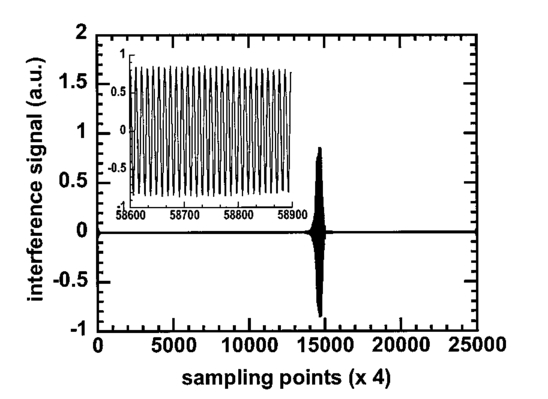

The error comes mainly from inaccurate setting of the variable wave plate. The actual parameters of the wave plate can be calculated from the measured Jones matrix. The retardation and the orientation of the wave plate were calculated to be 48.95° and −53.93°, respectively. The theoretically fitted roundtrip Jones matrix of a wave plate with the calculated retardation and orientation values (J _P2) and the relative amplitude and phase differences of the measured matrix from this theoretically fitted matrix ( J _ρd2 and J _φd2 ) are

\begin{matrix} J_{P 2} & = & [\begin{matrix} 1 & 0.343 - 0.972 i \\ 0.343 - 0.972 i & 0.779 + 0.627 i \end{matrix}] \\ = & [\begin{matrix} 1 & 1.031 exp (- 1.2316 i) \\ 1.031 exp (- 1.2316 i) & 1.0 exp (0.6777 i) \end{matrix}], \\ J_{ρ d 2} & = & [\begin{matrix} 0 & - 2.8% \\ - 2.8% & - 5.1% \end{matrix}], J_{φ d 2} = [\begin{matrix} 0 & 0.03% \\ 0.03% & 0.03% \end{matrix}] . \end{matrix}

4. Experimental Results and Analysis

The system was experimentally applied to image soft tissues. The first sample was a piece of porcine tendon. The tendon was mounted in a cuvette filled with saline solution. The sample was transversely scanned in steps of 5 μm and multiple A-scan images were taken. The digitized interference signals were band pass filtered, Hilbert transformed, and demodulated to extract the analytical signals of each component of the output Jones vectors. For each A scan, pixels were formed by averaging the calculated elements of the Jones matrix over segments of 1000 points. Two-dimensional (2D) images were formed from these A-scan images and then median filtered. Last, the amplitudes of the elements of the Jones matrix were pixelwise normalized with $\sqrt{M_{00}}$ and the phases were pixelwise subtracted by the phases of J₁₁. M₀₀ represents the intensity transformation from input light into output light and

Eq. (10)

M_{00} = \frac{1}{2} ({| J_{11} |}^{2} + {| J_{12} |}^{2} + {| J_{21} |}^{2} + {| J_{22} |}^{2}) .

The final 2D images of the Jones matrix J and M₀₀ are shown in Figure 3(a).

Figure 3

(a) M₀₀ and 2D Jones-matrix images of a piece of normal porcine tendon. (b) M₀₀ and 2D Jones-matrix images of the piece of porcine tendon heated for 20 s at 90 °C. (c) M₀₀ and 2D Jones-matrix images of a piece of porcine skin. (d) M₀₀ and 2D Jones-matrix images of a piece of bovine articular cartilage. The size of each image in (a) and (b) is 0.5 mm (width)×0.9 mm (depth). The size of each image in (c) and (d) is 1 mm (width)×0.9 mm (depth). Each image of the elements of the Jones matrix is pixelwise normalized with the corresponding $\sqrt{M_{00}}$ image and shares the same color table. The phase of each element is relative to the phase of J₁₁, which is zero with respect to itself. The M₀₀ images are on a logarithmic pseudocolor scale while the other images are on a linear pseudocolor scale.

Clear band structures can be seen in some of the images, especially in Re(J₂₂) and Im(J₂₂). There is no such band structure present in the M₀₀ image, which is the image based on the intensity of backscattered light. In other words, the M₀₀ image is free of the effect of polarization. We believe that the band structure is generated by the birefringence of the collagen fibers in porcine tendon. The band structure is distributed quite uniformly in the region measured; therefore, the birefringence is also uniform in the area measured.

After the test, the sample was thermally treated to test the change in polarization properties of biological tissue due to thermal damage. The sample was heated for about 20 s by touching it with a piece of metal, which was partially immersed in 90 °C water; the piece of metal was used for convenience in heating the sample in a specific area. The Jones matrix images shown in Figure 3(b) clearly show that the period of the band structure increased with the thermal treatment, which we believe is directly caused by the reduction of birefringence in the sample. This observation, birefringence loss caused by thermal damage, is consistent with the experimental result of another group.²¹

We also measured the images of the Jones matrix of a piece of fresh porcine skin [Figure 3(c)]. The skin sample was mounted in a cuvette filled with saline solution. Incident light was perpendicular to the surface of the skin. There is also some band-like structure in the images other than the image of M₀₀, which suggests the existence of birefringence. The structure is not as uniform as that of porcine tendon. The distribution and the orientation of the collagen fibers in porcine skin are apparently not as uniform as in porcine tendon. Only one period of the band-like structure can be seen, possibly due to the nonuniform distribution of the orientation of the birefringence.

The Jones matrix of a piece of bovine articular cartilage was also measured [Figure 3(d)]. In the images, the birefringence of the cartilage is apparently inhomogeneous from the surface down into the sample. It can be seen that the band structure is also inhomogeneous in the lateral direction. The inhomogeneous distribution of the band structure suggests that the orientation of the major axis, related to the fiber orientation of the sample, varies in the lateral direction.

Usually the parameters that characterize the polarization properties of a sample are contained implicitly in its Jones and Mueller matrices. Explicit polarization parameters of a sample, such as diattenuation, birefringence, and orientation of the fast axis, need to be extracted from the measured Jones or Mueller matrices through decomposition. For a nondepolarizing sample, the decomposition of its Jones matrix is equivalent to the decomposition of its Mueller matrix.

A Jones matrix can be decomposed by polar decomposition:¹³ ²²

Eq. (11)

J = J_{P} J_{R},

where J _P is the Jones matrix of a diattenuator (partial polarizer) and J _R is the Jones matrix of an elliptical retarder. In biological tissues, it is reasonable to believe that the orientations of the diattenuator and the retarder are the same because the orientations of both the diattenuator and the retarder are directly related to the orientation of the tissue fibers. In this case, J is homogeneous in the polarization sense²² and the order of J _P and J _R in Eq. (11) is reversible.

Because the effect of non-Faraday circular birefringence is cancelled in the roundtrip OCT signals and there is no Faraday circular birefringence without a magnetic field applied to the sample, only linear birefringence exists in Jones matrix J. We extracted polarization parameters from a piece of porcine tendon set at various orientations. The rotational axis of the sample is collinear with the optical axis of the incident light. The measurements were made at five different orientations at intervals of 10°. For a Jones matrix that contains linear birefringence and linear or circular diattenuation, the following relationships can be derived:

Eq. (12)

\begin{array}{l} Re (J_{11}) Im (J_{21}) - Im (J_{11}) Re (J_{21}) - Re (J_{12}) Im (J_{22}) \\ + Im (J_{12}) Re (J_{22}) = P (P_{1}, P_{2}) sin (2 θ) sin (φ) = M_{31}, \\ Re (J_{11}) Im (J_{22}) - Im (J_{11}) Re (J_{22}) - Re (J_{21}) Im (J_{12}) \\ + Im (J_{21}) Re (J_{12}) \\ = - P (P_{1}, P_{2}) cos (2 θ) sin (φ) = M_{32}, \\ M_{00} = \frac{1}{2} (P_{1}^{2} + P_{2}^{2}), \end{array}

where P is a function of P₁ and P₂. To increase the signal-to-noise ratio, every 20 adjacent A scans of M₃₁ and M₃₂ were averaged and the data corresponding to a physical depth of 0.4 mm from the surface (optical depth divided by the refractive index of the sample, which was assumed to be 1.4) were fitted for polar decomposition.

The averaged raw data and the fitted curves for the different orientations are shown in Figure 4. The evolution of M₃₁ and M₃₂ with the orientations can be clearly seen. The calculated birefringence from the fitted data is (4.2±0.3)×10⁻³, which is comparable with the previously reported value of (3.7±0.4)×10⁻³ for bovine tendon.⁷ The calculated birefringence of the thermally treated porcine tendon in Figure 3(b) is (2.24±0.07)×10⁻³, which is about half the normal value. After subtracting an offset, the calculated angles of the fast axis are shown in Figure 5. The small angular offset is due to the discrepancy between the actual and the observed fiber orientations. The results are very good considering that the tendon was slightly deformed when it was mounted in the cuvette and the rotational axis of the sample may not have been exactly collinear with the optical axis.

Figure 4

Averaged raw data of M₃₁ (^*) and M₃₂ (○), like in Eq. (12), of a piece of porcine tendon vs penetration depth and the fitted curve (—) for different orientations. From top to bottom the interval of variation of the orientation is −10°.

Figure 5

Calculated angle and standard error of the fast axis for different orientations of the sample in Figure 4.

The diattenuation is defined as

Eq. (13)

D = (P_{1}^{2} - P_{2}^{2}) / (P_{1}^{2} + P_{2}^{2}) = \sqrt{M_{01}^{2} + M_{02}^{2} + M_{03}^{2}} / M_{00},

where M₀₁, M₀₂, and M₀₃ are the elements of the corresponding Mueller matrix and can be calculated with Eq. (5). The D calculated was averaged over all the orientations and linearly fitted over a depth of 0.3 mm. The D fitted versus the roundtrip physical pathlength increases with a slope of 0.26/mm and reaches 0.075±0.024 at the depth of 0.3 mm after subtracting an offset at the surface.

The calculated birefringence of the porcine skin is mainly in the range of 1.5×10⁻³–3.5×10⁻³. The calculated birefringence of the bovine cartilage is about 3.0×10⁻³. The differences in Jones-matrix images among different samples are obvious. The magnitude of birefringence and diattenuation are related to the density and property of collagen fibers, whereas the orientation of the fast axis indicates the orientation of the collagen fibers. The amplitude and orientation of birefringence of porcine skin and bovine cartilage are not as uniformly distributed as in porcine tendon. In other words, the densities of collagen fibers in porcine skin and bovine cartilage are not as uniform as in porcine tendon, and the orientations of the collagen fibers are not distributed in as orderly a fashion as in porcine skin and bovine cartilage as in porcine tendon.

5. Conclusion

In summary, we developed a novel double-source double-detector polarization-sensitive OCT imaging technique. This technique enables the acquisition of a 2D tomographic Jones matrix, which can be converted into a Mueller matrix. The depth-resolved Jones matrix of a sample can be determined with a single scan; as a result, this technique is capable of imaging either hard or soft biological tissues. In addition, the Jones matrix can be decomposed to extract important information on the optical polarization properties of a sample, such as birefringence, orientation of the fast axis, and diattenuation. In our study, the Jones-matrix images of thermally treated porcine tendon clearly showed changes in birefringence due to thermal damage. The Jones-matrix images of different biological samples revealed that the polarization properties of different samples differ from each other although the birefringence in all of the samples was contributed primarily by collagen fibers. This technique has the potential to provide a new contrast mechanism for imaging biological tissues. Birefringence is sensitive to tissue changes because it is based on phase contrast.

Acknowledgments

This project was sponsored in part by National Institutes of Health Grant Nos. R21 RR15368 and R01 CA71980, by National Science Foundation Grant No. BES-9734491, and by Texas Higher Education Coordinating Board Grant No. 000512-0123-1999.

REFERENCES

1.

W. Drexler , U. Morgner , F. X. Ka¨rtner , C. Pitris , S. A. Boppart , X. D. Li , E. P. Ippen , and J. G. Fujimoto , “In vivo ultrahigh-resolution optical coherence tomography,” Opt. Lett. , 24 (17), 1221 –1223 (1999). Google Scholar

2.

I. Hartl , X. D. Li , C. Chudoba , R. K. Ghanta , T. H. Ko , and J. G. Fujimoto , “Ultrahigh-resolution optical coherence tomography using continuum generation in an air-silica microstructure optical fiber,” Opt. Lett. , 29 (9), 608 –610 (2001). Google Scholar

3.

G. J. Tearney , B. E. Bouma , and J. G. Fujimoto , “High-speed phase-and group-delay scanning with a grating-based phase control delay line,” Opt. Lett. , 22 (23), 1811 –1813 (1997). Google Scholar

4.

A. M. Rollins , M. D. Kulkarni , S. Yazdanfar , R. Ung-arunyawee , and J. A. Izatt , “In vivo video rate optical coherence tomography,” Opt. Express , 3 (6), 219 –229 (1998). Google Scholar

5.

J. M. Schmitt , “Restoration of optical coherence images of living tissues using the CLEAN algorithm,” J. Biomed. Opt. , 3 (1), 66 –75 (1998). Google Scholar

6.

M. Baskansky and J. Reintjes , “Statistics and reduction of speckle in optical coherence tomography,” Opt. Lett. , 25 (8), 545 –547 (2000). Google Scholar

7.

J. F. de Boer , T. E. Milner , M. J. C. van Gemert , and J. S. Nelson , “Two-dimensional birefringence imaging in biological tissue by polarization-sensitive optical coherence tomography,” Opt. Lett. , 22 (12), 934 –936 (1997). Google Scholar

8.

M. J. Everett , K. Schoenerberger , B. W. Colston Jr. , and L. B. Da Silva , “Birefringence characterization of biological tissue by use of optical coherence tomography,” Opt. Lett. , 23 (3), 228 –230 (1998). Google Scholar

9.

J. F. de Boer , T. E. Milner , and J. S. Nelson , “Determination of the depth-resolved Stokes parameters of light backscattered from turbid media by use of polarization-sensitive optical coherence tomography,” Opt. Lett. , 24 (5), 300 –302 (1999). Google Scholar

10.

G. Yao and L. V. Wang , “Two-dimensional depth-resolved Mueller matrix characterization of biological tissue by optical coherence tomography,” Opt. Lett. , 24 (8), 537 –539 (1999). Google Scholar

11.

S. Jiao , G. Yao , and L. V. Wang , “Depth-resolved two-dimensional Stokes vectors of backscattered light and Mueller matrices of biological tissue measured with optical coherence tomography,” Appl. Opt. , 39 (34), 6318 –6324 (2000). Google Scholar

12.

S. Jiao and L. V. Wang , “Two-dimensional depth-resolved Mueller matrix of biological tissue measured with double-beam polarization-sensitive optical coherence tomography,” Opt. Lett. , 27 (2), 101 –103 (2002). Google Scholar

13.

J. J. Gil and E. Bernabeu , “Obtainment of the polarizing and retardation parameters of a non-depolarizing optical system from the polar decomposition of its Mueller matrix,” Optik (Stuttgart) , 76 (2), 67 –71 (1987). Google Scholar

14.

E. Collett, Polarized Light Fundamentals and Applications, Chap. 10, Dekker, New York (1993).

15.

J. Li , G. Yao , and L. V. Wang , “Degree of polarization in laser speckles from turbid media: Implications in tissue optics,” J. Biomed. Opt. , 7 (3), 307 –312 (2002). Google Scholar

16.

F. Le Roy-Brehonnet and B. Le Jeune , “Utilization of Mueller matrix formalism to obtain optical targets depolarization and polarization properties,” Prog. Quantum Electron. , 21 (2), 109 –151 (1997). Google Scholar

17.

N. Vansteenkiste , P. Vignolo , and A. Aspect , “Optical reversibility theorems for polarization: Application to remote control of polarization,” J. Opt. Soc. Am. A , 10 (10), 2240 –2245 (1993). Google Scholar

18.

G. Yao and L. V. Wang , “Monte Carlo simulation of an optical coherence tomography signal in homogeneous turbid media,” Phys. Med. Biol. , 44 2307 –2320 (1999). Google Scholar

19.

Y. Zhao , Z. Chen , C. Saxer , S. Xiang , J. F. de Boer , and J. S. Nelson , “Phase-resolved optical coherence tomography and optical Doppler tomography for imaging blood flow in human skin with fast scanning speed and high velocity sensitivity,” Opt. Lett. , 25 (2), 114 –116 (2000). Google Scholar

20.

A. D. Poularikas, The Transforms and Applications Handbook, Chap. 7, Chemical Rubber, Boca Raton, FL (1996).

21.

J. F. de Boer , S. M. Srinivas , A. Malekafzali , Z. Chen , and J. S. Nelson , “Imaging thermally damaged tissue by polarization sensitive optical coherence tomography,” Opt. Express , 3 (6), 212 –218 (1998). Google Scholar http://epubs.osa.org/oearchive/source/5895.htm.

22.

R. A. Chipman, “Polarimetry,” in Handbook of Optics, Vol. II, Chap. 22, McGraw–Hill, New York (1995).

Citation Download Citation

Shuliang Jiao and Lihong V. Wang "Jones-matrix imaging of biological tissues with quadruple-channel optical coherence tomography," Journal of Biomedical Optics 7(3), (1 July 2002). https://doi.org/10.1117/1.1483878

Published: 1 July 2002

Access the abstract

JOURNAL ARTICLE
9 PAGES

DOWNLOAD PAPER SAVE TO MY LIBRARY

GET CITATION

CITATIONS

Cited by 144 scholarly publications and 41 patents.

Explore citations on Lens.org

RIGHTS & PERMISSIONS

Get copyright permission Get copyright permission on Copyright Marketplace

KEYWORDS

Polarization

Optical coherence tomography

Birefringence

Tissues

Jones vectors

Light sources

Wave plates

1.

Introduction

2.

Jones Matrix and Mueller Matrix