1.IntroductionMultiphoton laser-scanning microscopy (MPLSM) utilizes infrared ultrafast laser pulses (generally femtosecond range), allowing very large instantaneous intensities to be attained in a diffraction-limited focal volume. Within this femtoliter volume, the transient intensity is sufficiently high to increase the probability of simultaneous absorption of multiple (n) long-wavelength photons substituting for the absorption of single photons of n times the energy, in accordance with the theory of Go¨ppert-Mayer.1 The use of this multiphoton effect has proven invaluable in microscopic imaging of biological specimens, such as living brain slices, which are optically thick (300 to 500 μm) light-scattering specimens, owing to its significantly increased penetration depth and reduced volume of fluorescence excitation.2 For example, multiphoton microscopy has been applied to high-resolution structural imaging applications, such as the observation of activity-induced changes in dendritic spine shape,3 as well as functional imaging applications, where optical signals are recorded that track physiological processes in cells, such as the measurement of Ca 2+ transients within individual dendritic spines.4 One technical factor, however, has limited the efficacy of MPLSM, particularly for functional imaging applications. Commercial multiphoton systems generally employ inertia-limited galvanometer-driven mirrors to scan the laser beam across the field of view. Therefore, in time-critical functional imaging applications, users generally resort to single line scans, configured to cross-sites of interest to achieve sufficiently high frame rates for tracking the physiological process of interest (e.g., transient intracellular calcium elevations that last for less than 100 ms). This approach is disadvantageous for several reasons: 1. achievable frame rates are limited to ∼100 Hz, even with the sacrifice of one scan dimension; 2. potential signal integration time at sites of interest is wasted due to continuous beam movement; and 3. line scans do not conform well to the intricate shapes of biological structures, particularly neuronal or vascular arborizations. These limitations can be overcome through the use of acousto-optic deflectors (AODs), which provide inertia-free beamsteering, allowing for fast (1 to 10 μs) repositioning from any point in the field of view to any other. These devices employ high-frequency sound waves in a crystal, which conceptually act as a tunable diffraction grating [Fig. 1(a)]. As shown, adjusting the acoustic frequency effectively varies the grating constant, altering the beam deflection angle. By employing two orthogonal AODs, a random-access x-y scanner can be fashioned. Using such a scanner, the user can select multiple sites of interest and sample them repeatedly at very high frame rates (>1 kHz).5 6 In addition, for a given frame rate, the dwell times at the sites of interest can be made greater than possible with a (continuously moving) line scan system, increasing the signal strength and thus the achievable signal-to-noise ratio [Fig. 5(b)]. Figure 1Acousto-optic scanning principle. (a) Scan angle θ(t) and output intensity I1(t) of a laser beam in the first diffraction order of an AOD controlled by frequency f(t) and amplitude V(t), of an acoustic wave in the AO medium. Remainder of input intensity (I) is left undeflected in the zeroth diffraction order (I0). (b) Scheme of individual nerve cell with user-selected sites of interest imaged by random-access scanning at very high frame rates (>1 kHz).  The advantages of AO scanning are considerable, even when compared to specialized noncommercial fast-scanning schemes that have been developed for MPLSM. Some schemes have pushed the limits achievable with inertial galvanometric-based scanning. These include optimized driving voltages for normal galvanometers to achieve fast (>100 Hz) single region of interest (∼25 μ m 2) scans,7 and the use of resonant galvanometers to reach fast (up to 240 Hz) full field-of-view scanning.8 However, neither approach allows multiple, noncontiguous sites of interest to be imaged at such high frame rates with optimal integration times at each, as AO scanning permits. Another fast-scanning technique—multifocal multiphoton microscopy (MMM)9 10 11—has allowed fast imaging (up to 3 to 4 kHz in one implementation9). This approach is limited, however, in that it cannot collect all emission from sites of interest. Also, it is limited to either full-field scans (and its intrinsically short dwell times) in the Nipkow disk implementation,9 or to rigid illumination patterns (which may not match the sites of interest) in the fixed microlens array systems.10 Furthermore, MMM approaches are apt to be power limited and require imaging detectors, which can be complex to align with the illumination pattern, are frame-rate limiting, and cannot match the performance of the best nonimaging detectors. Despite the instrumental advantages and the experimental potential, AO scanning has only just recently been integrated with multiphoton microscopy in a hybrid AO-galvanometer scheme.12 In general, the combination of AO scanning and MPLSM has been avoided because AODs are typically made from highly dispersive materials, and therefore induce significant spatial and temporal dispersion (pulse broadening). Spatial dispersion results in larger focal volumes, reducing the spatial resolution achievable with an AO-MPLSM; temporal dispersion increases the laser pulsewidth, significantly decreasing the probability of multiphoton excitation. We describe the problems of spatial and temporal dispersion and present novel strategies for compensating each, specifically applied to the development of a 2-D AO-MPLSM system. Spatial dispersion is not a well-documented phenomenon, so we present here calculations showing the effect to be significant (up to ten-fold) for a high-resolution AO-MPLSM application. We introduce a compensation scheme, previously documented in conference proceedings,13 based on a single additional diffraction grating per AOD. Such a scheme is shown to eliminate the spatial dispersion at the center of the field of view and reduce it by no less than three-fold elsewhere. In contrast, the recent work by Lechleiter, Lin, and Sieneart12 employed a prism, instead of a diffraction grating, to compensate the spatial dispersion of a single AOD in their hybrid AO-galvanometer scanner. While this research showed high-resolution MP images, it did not present a detailed calculation or demonstration of the dispersion effect’s severity for an MPLSM application. We provide a direct measurement of spatial dispersion for a custom-made AOD designed specifically for high-resolution 2-D MPLSM, establishing the importance of spatial dispersion compensation. A demonstration of the grating-based dispersion compensation is also provided. Temporal dispersion compensation has been well documented elsewhere and involves the use of a negative-GVD introducing prechirper.14 15 Because of the especially large group-velocity dispersion (GVD) associated with a system involving two highly dispersive AODs, the path length required for a standard prism-pair prechirper can become excessive (>3 m) for many laboratory settings. We have thus devised a novel stacked prism prechirper geometry, which reduces by two-fold the required physical path length. 2.Spatial Dispersion Compensation2.1.BackgroundAODs are often regarded as tunable diffraction gratings. By varying the acoustic frequency, the grating constant can be altered, allowing a monochromatic laser beam to be steered. For a typical AOD operating in the Bragg regime, the deflection angle of the beam is given by where λ is the optical wavelength, Λ is the acoustic wavelength, f is the acoustic frequency, and v acoustic is the acoustic velocity in the AOD.Ultrafast laser pulses, however, are not monochromatic and are thus dispersed by this acoustic diffraction grating. This phenomenon can be termed spatial dispersion, or spatial chirp, to distinguish it from temporal dispersion. It is manifest as an angular broadening of the beam (Δθ beam ) that limits the spatial resolution of the AOD, which is generally specified in terms of the AOD’s time-bandwidth product N. This quantity reflects the number of distinct resolvable spots in the far field, which directly translates into the number of resolvable spots in the microscope objective’s field of view, The quantity Δθ scan represents the angular range over which the AOD can deflect the laser beam as the frequency is tuned. Derived from Eq. (1), Δθ scan is simply proportional to the acoustic bandwidth of the AOD driver Δf, Meanwhile, Δθ beam could be termed the angular spread of the laser beam, which, in the absence of spatial dispersion, is determined by the diffraction limit imposed by the AOD aperture size d, The published specifications of a particular AOD generally contain a value for N calculated as N=Δθ scan /Δθ beam,diffraction . For ultrafast laser pulses, the effect of spatial dispersion is to increase the value of Δθ beam . Hence, the angular spread of an ultrafast laser beam is simply In a situation where Δθ beam,dispersion is significantly greater than Δθ beam,diffraction , the time-bandwidth product N is accordingly reduced and the spatial resolution can be said to be dispersion, rather than diffraction-limited.2.2.Slow-Shear TeO2 AODsTypical biomedical applications of an AO-MPLSM involve imaging very small cellular structures—for instance the dendritic spines found on many neurons—which are <1 μm in size. As an estimate of the required resolution, the field of view of a typical 60× water-immersion objective used for brain slice imaging is ∼300 μm. The best (diffraction-limited) lateral resolution possible, assuming some typical conditions—λ=900-nm excitation and an objective lens with NA=1.0—is ∼450 nm, i.e., λ/(2NA). An ideal AO-MPLSM would permit diffraction-limited imaging throughout practically the entire field of view. Using these numbers as a guideline, a resolution of N∼500 spots is a good estimate of the required AOD performance. Commercial AODs made of tellurium dioxide (TeO 2) are readily capable of providing such resolution. TeO 2 deflectors can be designed to either employ a longitudinal or slow-shear acoustic wave mode. The former mode is faster (v acoustic ∼4200 m/s) and can support large frequency bandwidths (Δf∼200 MHz), while the latter mode is slower (v acoustic ∼650 m/s) but restricted to operate at lower acoustic frequencies (to satisfy the off-axis angle requirement particular to shear-mode acoustic waves to avoid a dip in the diffraction efficiency across the scan bandwidth16). For Ti:S laser wavelengths (e.g., λ0=850 nm), a central frequency of f0=70 MHz is indicated, which practically—considering limitations in transducing an effective phased array acoustic field—allows an acoustic frequency bandwidth of Δf=f0/2=35 MHz. 17 Applying Eq. (3), this implies that the slow-shear mode offers 1.3× greater spatial resolution per unit of beam diameter (d), compared to the longitudinal mode. Such a modest benefit weighed against the significantly faster (6.5×) positioning time (scales inversely with v acoustic ) of the longitudinal mode device would seem to argue that this mode is preferable. Indeed, the recently developed system employing 1-D AO deflection for MPLSM12 adapted a commercial (Oz; Noran) unit containing a single longitudinal mode TeO 2 AOD. However, longitudinal mode devices such as this one are not well suited for extension to a 2-D AO scanning system, which is necessary to achieve the benefits of random-access scanning. The acousto-optic figure of merit of longitudinal TeO 2 devices is inferior to that of slow-shear TeO 2 devices, which causes two difficulties for the extension to 2-D AO scanning. First, the diffraction efficiency is greatly reduced (∼25 at the center position for 850 nm) and, second, these devices necessarily have a very thin rectangular aperture (∼0.5 mm), forcing the user to employ cylindrical optics. A robust cylindrical optics 2-D AO scanning system is far more complex to develop. For these reasons, a custom-made slow-shear TeO 2 device with high diffraction efficiency (>70 at peak) and a large square aperture was used for the work here. Using such devices, a 2-D AO-MPLSM system can be constructed following a spherical optics design similar to that previously employed in our laboratory.5 6 2.3.Spatial Dispersion of Custom Slow-Shear TeO 2 AODThe custom-made AOD (ATD-7010CD2; IntraAction) has a large active aperture of 10×10 mm. Given the acoustic bandwidth Δf=35 MHz and the slow-shear acoustic mode velocity of 660 m/s, the angular range Δθ scan is 45.1 mrad at an optical wavelength of 850 nm. Meanwhile, applying the sinc 2 [(πd/λ)θ] form for diffraction at a rectangular aperture, an angular spread of Δθ beam,diffraction =0.88λ/d=75 μrad, is found for λ=850 nm, using the full-width half maximum (FWHM) to define the beam angular width (somewhat more relaxed than customary Rayleigh criterion). Computing the time-bandwidth product N=Δθ scan /Δθ beam , a spatial resolution figure of N∼600 spots is obtained in the absence of dispersion. To what extent would spatial dispersion worsen this spatial resolution? Applying Eq. (5) at the center of the scan angle range, we find the dispersed beam’s angular spread to be Elsewhere, the amount of spatial dispersion varies across the field of view linearly, such that at the two extreme borders of the scan pattern. These cases are depicted in Fig. 2.Figure 2Spatial dispersion by AOD. Spatial dispersion of an ultrafast laser pulse over angle Δθ beam , limiting the number of resolvable spots across the angular range Δθ scan . The amount of beam dispersion grows linearly with the scan angle for increasing acoustic frequencies.  Assuming Gaussian pulse shapes, a 130-fs (FWHM) pulse (the specification pulsewidth of the Mira900D laser primarily used here) implies that Δλ∼8 nm (FWHM), following the 0.441 time-bandwidth product (ΔtΔν) for the Gaussian pulse shape.18 Applying f0=70 MHz, one finds Δθ beam,dispersion =740 μrad (FWHM) at the center of the scan pattern. This is approximately ten times worse than Δθ beam,diffraction . Thus, the spatial resolution is limited to only ∼60 spots, or >5 μm when filling the field of view of a typical 60× objective. Figure 3(a) compares the calculated angular distributions for the diffraction- and dispersion-limited cases. Figure 3Spatial dispersion by custom-made TeO 2 AOD. (a) Computed angular beam width due to diffraction (solid) at overfilled 10×10-mm AOD aperture and dispersion (dotted) of the laser’s nominal 130-fs pulsewidth. Dispersion is predicted to worsen spatial resolution by ∼10×. (b) Measured intensity distribution of focused spots of deflected Ti:S beam, with a laser in continuous wave (CW) and modelocked (ML) modes. Spatial dispersion of femtosecond pulses (ML) leads to a 2.8× broadening of focused spot size. (c) Two-spot scan patterns demonstrating severely compromised lateral spatial resolution with ultrafast pulses (ML mode). 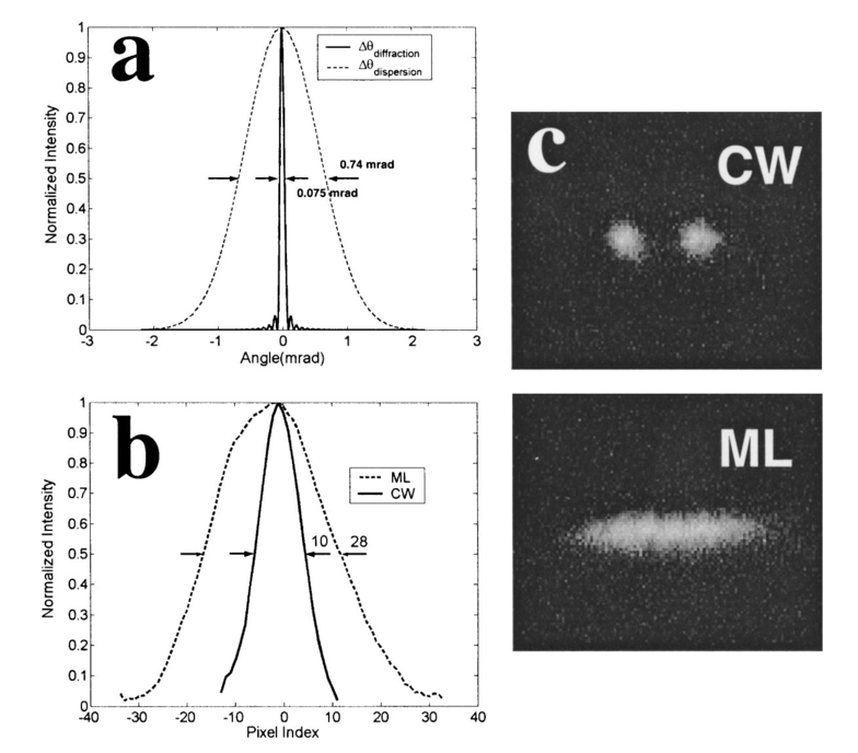 We verified the presence of spatial dispersion using one such custom slow-shear TeO 2 device, overfilling its 10×10-mm aperture with an expanded and spatially filtered beam from a commercial Ti:S laser (Mira 900D; Coherent), tuned to 850 nm. The AOD was driven by a voltage-controlled oscillator (DE-702M; IntraAction). First, the acoustic frequency was tuned to a constant value near the central frequency f0 (70 MHz), and the resulting deflected beam was focused onto a distant screen at an angular magnification of 2.5×. Figure 3(b) shows smoothed (eight-point moving average) line sections through captured video images [not shown, but similar to those in Fig. 3(c)] of the focused spot when the laser was alternately operated in mode-locked (ML), i.e., femtosecond-pulsed, and continuous wave (CW) modes. The ML mode spot had a 28-pixel-wide FWHM, compared to 10 pixels FWHM for the CW mode spot. Next, the acoustic frequency was switched rapidly between two closely spaced acoustic frequencies (Δf∼800 kHz) about the center frequency f0 (70 MHz) to produce a two-spot scan pattern. The resulting video images of the focused scan patterns in CW and ML modes are shown in Fig. 3(c). While the spots are clearly resolvable in CW mode, they are entirely indistinguishable in ML mode. The observed dispersion effect (2.8×) was less than that predicted, owing to aberration-limited focusing of the spots. Nevertheless, these tests reveal that spatial dispersion does indeed significantly limit the achievable resolution of an AO-MPLSM system, when uncompensated. 2.4.Spatial Dispersion CompensationTo remedy this, we have employed a compensation scheme based on a single diffraction grating that significantly reduces this dispersion-induced spatial broadening. This compensation grating, inserted directly after the AOD, has a grating constant matched to the central acoustic frequency of the AOD and is configured to diffract efficiently in the opposite diffraction order compared to the AOD (i.e., the -1 order). This scheme is depicted in Fig. 4. Without the grating, as shown in Fig. 4(a), the focused spots are broadened in a linearly varying fashion across the field of view. With the practical assumption that the acoustic bandwidth Δf≈f0/2, the spot size varies linearly from its minimally broadened value s at f min to 1.67s at f max , as shown in Fig. 4(a). By employing the diffraction grating, as shown in Fig. 4(b), the scan angles are realigned with the original optical axis and, more importantly, the dispersion Δθ beam,dispersion is uniformly reduced throughout the scan range by Δλf0/v acoustic . Thus, from Eq. (6), the separated spectral components are brought exactly back together at the central scan position, so that Further, throughout the rest of the scan range, the residual Δθ beam,dispersion is significantly reduced; following Eq. (7), we find at both borders of the scan range. Comparing Eqs. (7) and (9) in the practical case, where Δf≈f0/2, it is found that the maximal compensated spot size is one-third that of the smallest spot size in the uncompensated pattern. Thus, as shown in Fig. 4(b), the spot sizes in the compensated pattern vary linearly from diffraction limited in the center to 0.33s at both borders. The absolute value in Eq. (9) reflects the fact that the sign of the dispersion is reversed on the low-frequency side of the range, i.e. the wavelengths are inverted, as shown by the crossing of the red and blue rays in Fig. 4(b). Note also that these results are insensitive to laser wavelength λ0.Figure 4Spatial dispersion compensation. (a) Uncompensated deflection of ultrafast laser pulse by AOD results in broadened spot sizes (s to 1.67s) in the specimen plane. (b) Single diffraction grating matched to a central acoustic wavelength eliminates spatial dispersion in the center of a scan pattern, with maximal residual dispersion of 0.33 s at the borders. Note the direction of the residual spatial dispersion is reversed for acoustic frequencies below central value (f0) (c) Demonstration of spatial dispersion compensation using a second AOD with a counterpropagating acoustic wave tuned to a central frequency of the first AOD. The multiline Ar laser acts as broadband source (488 to 514 nm).  In summary, the extent of the predicted compensation can be quantified as, at minimum, a three-fold improvement relative to the uncompensated pattern. The improvement is five-fold at the other scan pattern border and is maximal at the center of the pattern. These values assume that the spatial dispersion effect leads to a large (>5×) broadening throughout the field of view, as in the case of 10× broadening for the custom-made TeO 2 previously described [Fig. 3(a)]. In this specific case of employing a large-area slow-shear TeO 2 AOD and filling the field of view of a high-NA objective lens, the compensation grating would restore the spatial resolution to ∼1 μm near the borders of the field of view, while allowing the full diffraction-limited resolution at the center. We tested this scheme for dispersion compensation by employing the two main lines of a multiline argon laser (488 and 514 nm) to model the extremes of the broadened spectrum of an ultrafast pulse. These lines were passed through a PbMbO 4 deflector (1205C-2; Isomet), driven by a repeating staircase of five frequencies to produce a simple five-spot scanning pattern. The compensation grating was fashioned from a second identical AOD, which was tuned to the central frequency of the first (scanning) AOD, and oriented in the opposite direction (i.e., the acoustic waves were counterpropagating). Figure 4(c) shows the 0 (uncompensated) and -1 (compensated) diffraction orders that passed through the second AOD. The compensation was highly effective, allowing the five-scan positions to be clearly distinguished where they could not be without compensation. 3.Temporal Dispersion Compensation3.1.BackgroundTemporal dispersion refers to the broadening of ultrashort pulses propagation through dispersive materials, i.e., those with a frequency-dependent index-of-refraction n(ω). On traversing a medium of length L, light of a particular frequency ω is phase shifted by an amount ϕ The accumulation of phase per unit length is given by the wavenumber k=ϕ(ω)/L. Differentiating twice with respect to ω and expressing the results in terms of the vacuum wavelength λ yields The term on the left can be viewed as the accumulation of second-order phase per unit length. It is also referred to as the GVD constant D, and is often given in units of fs 2 /cm.By the Fourier theorem, a pulse of light is necessarily composed of several wavelengths. Within this pulse spectrum, each infinitesimally small group of wavelengths travels at a group velocity given by dω/dk. The GVD of a material reflects the variation in group velocity across the spectrum, usually such that higher frequencies travel at slower group velocities, causing the pulsewidth to broaden. Assuming an input pulsewidth of τin, a GVD constant D, and a propagation length L, the output pulsewidth τ out is given by18 where the factor of 7.68 arises from the assumption that the pulses are Gaussian in shape and that the pulsewidths are specified in terms of the FWHM.In an MPLSM system, the aggregate material GVD of all the optics in the path—particularly the objective lens—yields a broadened pulsewidth at the specimen focus. As the average power required to maintain a fixed multiphoton excitation (and hence emission) rate scales as τ(n−1)/n, broadened pulses force the user to employ higher average powers.19 This accelerates the rates of photodamage and photobleaching, reducing the useful experimental time. 3.2.Temporal Dispersion by Slow-Shear TeO2 AODIn a typical mirror-based scanning system, a total GVD of up to ∼5000 fs 2 may be found,15 which has only a modest effect on the ∼100-fs pulses obtained from most commercial Ti:S oscillators. In comparison, an AO-MPLSM would incorporate two AODs, each of which gives rise to more than 10,000 fs 2 of GVD. This is due to the large GVD constants of the AO media employed for visible and near-IR wavelengths— PbMbO 4 and TeO 2 —as well as their long interaction path length (2 to 4 cm), which are necessary to achieve an adequate diffraction efficiency. We measured the GVD of one of the custom-made slow-shear TeO 2 AODs previously discussed, using a commercial autocorrelator that employs a two-photon absorption GaAsP photodiode (Mini-Microscope Autocorrelator; APE Berlin). In Fig. 5(a), a pair of interferometric autocorrelograms are taken using a commercial Ti:S laser (Mira 900D; Coherent) at λ=840 nm with and without the (undriven) AOD positioned before the autocorrelator. The characteristic rising of the “pedestal” associated with significant temporal chirp (i.e., dispersion) is evident in the lower (AOD+) figure. Because it is difficult to extract quantitative information about pulsewidths from such interferometric traces, we employed the instrument’s filter function to eliminate the fringes and the pedestal characteristic, revealing intensity autocorrelograms such as those shown in Fig. 5(b), also taken at λ=840 nm. The FWHM of these traces, obtained by a parametric fitting of an assumed Gaussian shape, was used as a robust measure of the pulsewidth. We obtained such values with and without the AOD at 20-nm intervals from 760 to 880 nm. Assuming a Gaussian laser pulse shape, the actual pulsewidths (stated as the FWHM) can be calculated as 0.71 times the measured autocorrelation FWHM pulsewidths.18 From the original and dispersed pulsewidths and the AOD’s known path length (L=2.79 cm), the GVD parameter D was calculated at each wavelength using Eq. (12). The measured values, shown as the data points in Fig. 5(c), follow a decreasing trend toward greater wavelengths. The Gaussian pulsewidths measured at each wavelength and the calculated values of D are given in Table 1. The intracavity prism pair of the laser was adjusted to produce the minimal pulsewidth for each wavelength, and pulses substantially shorter than the manufacturer’s specification of 130 fs were obtained at most wavelengths. Figure 5Temporal dispersion of custom TeO 2 AOD. (a) Measured interferometric autocorrelograms of laser pulsewidth without (AOD-) and with (AOD+) deflector, λ=840 nm. Effect of temporal dispersion is evident in the rising of a pedestal in the AOD+ case. (b) Measured intensity autocorrelogram without (AOD-) and with (AOD+) deflector present. Laser pulses are presumed Gaussian-shaped with a FWHM of 0.71×. (c) Dispersion (GVD) parameter computed from data such as in (b) at various laser wavelengths shown. The predicted GVD parameter is based on Sellmeir coefficients for the ordinary (solid) and extraordinary (dotted) indices of refraction of TeO 2.  Table 1
We compared these values to a theoretical curve determined by employing published Sellmeir equations20 for both the ordinary (n0) and extraordinary (ne) indices of refraction of TeO 2, There are two indices of a fraction because TeO 2 is a positive uniaxial crystal. The GVD parameter (d2k/dω2) was determined according to Eq. (11) using second derivatives n″(λ) of these indices. The lines in Fig. 5(c) show the values calculated across the Ti:S tuning range (700 to 950 nm) for the ordinary (solid) and extraordinary (dotted) axes. The measured GVD values follow a downward trend similar to these calculated curves, tracking most closely the computed extraordinary index of refraction. In fact, the incident optical wave in slow-shear TeO 2 devices propagates nearly along the optical axis and should thus propagate more nearly according to the ordinary index.16 Thus, the measured dispersion was modestly larger than theory would predict, but similar in magnitude and trend.The amount of dispersion, both measured and theoretical, was significant. Each AOD has a path length of 2.8 cm, so it is apparent that a pair of AODs would by themselves give rise to ∼30,000 fs 2. Under such conditions, an input pulsewidth of 100 fs (similar to those we measured in the 820 to 860 nm tuning range) would be broadened by ∼8×, which would necessitate a nearly three-fold increase in average power to maintain the same fluorescence yield. 3.3 GVD Compensation: Prechirper PrincipleTo avoid a marked increase in the requisite incident power, it is desirable to add an adjustable amount of negative GVD in the optical path to compensate for the temporal broadening caused by material dispersion. This is typically achieved by employing either diffraction gratings21 or dispersive prisms.22 Such devices for adding negative GVD are often referred to as prechirpers. Both gratings and prisms are spatially dispersive elements—they deflect different wavelengths of light by varying angles—by virtue of diffraction and refraction, respectively. Using either mechanism, prechirpers force longer wavelengths to travel through a longer optical path length, thereby reversing the temporal broadening incurred by the positive material GVD. The canonical layout of such prechirpers is shown in Fig. 6, in which four of each dispersive element are employed. In both cases, the first element disperses the light as a function of wavelength, such that longer wavelengths traverse a longer distance through glass (prisms 2 and 3) in the prism case, or a longer distance through air in the grating case. The lengths of the converging and diverging regions labeled in the schemes must be identical to cancel out the spatial chirp introduced by the first dispersive element. However, the combined value of this length L can be adjusted to vary the amount of negative GVD—the greater the length, the greater the separation of wavelengths. 6Schemes of canonical prechirpers. Either reflection gratings (a) or prisms (b) can be used as dispersive elements. In both schemes, beams are dispersed by the first element and then propagate over L/2 to separate wavelengths. Longer wavelengths are delayed by traveling longer paths. Wavelengths are recombined by a third element, followed by another L/2 propagation. Changing the total converging/diverging distance L adjusts the amount of negative GVD. 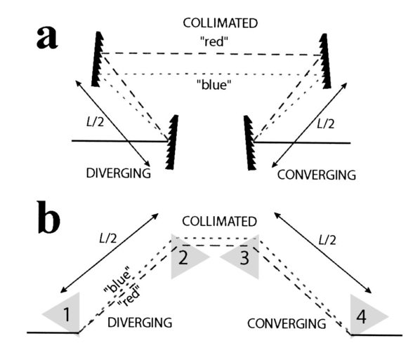 Since optical gratings can be made much more dispersive than prisms, the total path length of a grating-based prechirper is typically much shorter than a prism-based one for a given amount of GVD compensation. However, prisms offer two important advantages. First, they are more transmissive, approaching 99 when used at Brewster’s angle incidence, whereas grating efficiencies rarely exceed 80 (which leads to only 0.84, or ∼40, transmission on four reflections, compared to >90 with prisms). Second, when used in a minimum-deviation configuration, each of the prisms in Fig. 6(a) can be translated without affecting the optical path between the prisms. Since the path length through the prisms is a source of positive GVD, the total GVD can be continuously tuned by the addition and removal of glass. This degree of freedom adds a fine GVD control to the prechirper. For these important reasons, prism prechirpers are the method of choice where possible. Based on the analysis of Fork, Martinez, and Gordon,22 the negative GVD imparted by a prism prechirper is given by where L is again the total interprism path length through air in the converging and diverging regions of Fig. 6. Compared with Eq. (11), note that the negative GVD depends on the first-order dispersion of the prism dn/dλ, whereas the positive GVD depends on the second-order dispersion d2n/dλ2 of all the optics in the optical path. To keep the total interprism spacing L to a minimum, prism materials with large first-order dispersion are used, such as SF10 Schott glass. Employing readily obtained Sellmeir coefficients to calculate dn/dλ for SF10 at various wavelengths, the total interprism spacing L required to compensate for two of the custom-made TeO 2 AODs was computed. The results are given in Table 2. The GVD values are the theoretical ones associated with the ordinary index of refraction from Fig. 5(c).Table 2
At all wavelengths, the total interprism path length L required is ∼3 to 4 m. This does not include the extra length that would be required to compensate for the positive GVD imparted by other optical glass including the objective lens and the SF10 prisms themselves. The large physical footprint implied by large interprism spacings can be cumbersome, particularly in a biomedical laboratory setting, where space is often more critical than in a physics laboratory. Therefore, it is desirable to devise geometries that significantly reduce the prechirper’s physical size. 3.4.Space-Saving Geometry: Stacked-Prism PrechirperAs shown in Fig. 7(a), a plane of mirror symmetry exists between the second and third prisms in the canonical four-prism design. This is generally exploited by placing a roof mirror assembly at that plane, which reflects the beam along the same path as the incident beam, but at a different optical height. This results in the situation shown in Fig. 7(b), where the number of prisms and the physical interprism path length are both reduced by a factor of 2 by directing the beam a second time between prisms 1 and 2. Figure 7Space-saving prism prechirper schemes. (a) Canonical four prism sequence. (b) Common scheme with 50 reduced physical path length using a roof mirror at the plane of mirror symmetry in (a), requiring only two prisms. (c) Novel scheme with another 50 reduction of physical path length by insertion of another roof mirror at the folding plane in (b), and vertically stacking the prisms.  Because of the exceptional length L (3 to 4 m) required to compensate for a pair of TeO 2 AODs, we endeavored to reduce the physical path length even further. To achieve this, we devised the stacked prism prechirper geometry in which an additional roof mirror assembly was placed at the midpoint between the two prisms in Fig. 7(b), to create the situation shown in Fig. 7(c). The second prism is now located above the first prism (stacked) and rotated to deflect the beam into a separate short arm that contains the collimated region. The beam now traverses the distance between the two prisms four times, and thus the physical path length (of the longest dimension) is reduced by an additional factor of 2. The stacked-prism design is shown in more detail in Fig. 8. The structure forms a Y shape [Fig. 8(a)], with the input/output section forming the tail, and the long and short arms of the Y corresponding to the converging/diverging regions (B,D) and the collimated region (C) of the canonical four-prism prechirper depicted in Fig. 8(b). The beam travels at four separate heights through the long arm, which are enumerated in relation to the canonical four-prism design in Fig. 8(b). The height steps are made by the customary roof mirror assembly (region C) located at the end of the short arm and the additional roof mirror, termed the periscope assembly, located at the end of the long arm. Figure 8Stacked-prism pair prechirper design. (a) Mechanical layout of Y-shaped stacked-prism prechirper. Conceptual locations of prisms, roof mirror, and periscope mirror assemblies are indicated, according to a canonical four prism prechirper shown in (b). Heights of beam propagation in each segment are indicated by circled numbers. Labeled regions A through E are referred to in text. (c) Photographs of stacked prism prechirper. Note that two alignment tools, each with holes at the four optical heights (a, b), are inserted in the long arm. Long and short arms can be rotated relative to prism assembly during alignment. (d) Prism assembly. Prisms on translation stages are mounted onto tilt/rotation stages. (e) Roof mirror assembly. (f) Periscope assembly. The beam passes at all four optical heights. This assembly translates on the long arm to adjust the amount of negative GVD.  The prechirper was aligned through the use of two custom alignment tools that were inserted at two separated points in the long arm. Mirrors were adjusted so that the beam propagated through two separated pinholes at each of the four optical heights. Once aligned, the amount of negative GVD imparted by the stacked-prism prechirper could be adjusted by translating the periscope assembly along the long arm to vary the total interprism spacing L, with little to no beam realignment. The prisms in the central assembly were each located on translation stages, which allowed glass to be added and removed at each level (primarily the lower one is used, as the beam is not spatially dispersed there) as an effective fine-tuning knob for the GVD compensation. Referring back to Table 1, the additional two-fold reduction in physical path length provided by the stacked-prism prechirper design presented here allows the length of the long arm to be kept <1 m, for the entire Ti:S tuning range, for the compensation of two of the custom TeO 2 AODs described. Such a length can be accommodated by most optical tables, with sufficient room to spare for other equipment. 3.5.GVD Compensation DemonstrationWe tested the stacked-prism prechirper using a Ti:S laser (Kapteyn-Murnane Laboratories Kit) tuned to ∼780 nm. An interferometric autocorrelator based on a GaAsP photodiode that exhibits multiphoton conductivity (FR-103PD; Femtochrome Research) was employed. The interference fringes were filtered out, producing an intensity autocorrelogram (with background). Figure 9 shows four autocorrelation traces illustrating the effect of GVD compensation. The traces were measured in the absence or presence (AOD-/AOD+) of a single PbMoO 4 AOD (1205C-2; Isomet). The distance L phys of the periscope assembly from the central prism assembly along the long arm was set to be either short (COMP-: L phys =25 cm) to self-compensate for the prechirper’s prisms (fully inserted), or longer (COMP+: L phys ∼60 cm) to compensate for the additional GVD from the deflector. Figure 9GVD compensation with stacked-prism pair prechirper. Intensity autocorrelograms of Ti:S laser pulses acquired with a GaAsP photodiode-based autocorrelator. Lengths L phys reflect the distance from the periscope assembly to the prism assembly on the long arm. COMP-/AOD-: L phys =25 cm; AOD removed. The prechirper is self-compensated, producing net zero-GVD, revealing ∼240-fs autocorrelation trace of laser pulsewidth. COMP-/AOD+: L phys =25 cm; single AOD was added. Autocorrelation trace broadened to ∼800 fs (FWHM). COMP+/AOD-: L phys =62 cm; AOD removed. Prechirper provided large uncompensated negative GVD, yielding equally broadened autocorrelation trace. COMP+/AOD+: L phys =55 cm; AOD inserted. Negative and positive GVD balance, restoring original pulsewidth. 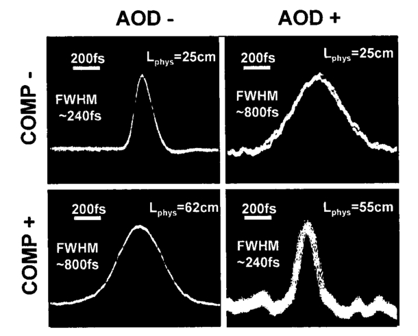 The AOD-/COMP- case represents the original laser pulsewidth, as verified in a separate measurement with the prechirper entirely removed. The FWHM observed was ∼240 fs, reflecting a Gaussian pulsewidth of ∼170 fs. This pulsewidth was somewhat long for this cavity and likely reflected a nonoptimal GVD of the intracavity prechirper. Alternatively, temporal filtering of the photodiode signal employed to improve the signal-to-noise ratio may have contributed to this broadening. Insertion of the AOD increased the measured pulsewidth to ∼800 fs (AOD+/COMP-), or ∼570 fs for the underlying Gaussian. This broadening corresponds to a total GVD of ∼12,000 fs 2, which is similar in magnitude to that provided by a single TeO 2 device. The AOD-/COMP+ case showed that the same broadened pulse could be observed with a long interprism path length in the absence of the AOD, demonstrating that both positive and negative GVD of the same quantity yield the same temporal broadening. Finally, the AOD+/COMP+ case revealed that positive and negative GVD can be combined to restore the original pulse width. These results demonstrate that the stacked-prism prechirper provides the large amounts of negative GVD required to fully compensate the GVD of this commercial AOD, with a relatively short physical path length of only 30 cm. Its GVD was comparable in magnitude to that of the custom TeO 2 devices suited for an AO-MPLSM system. Thus, GVD compensation of two TeO 2 AODs with a prism pair separated by <1 m is readily feasible with the stacked-prism design. 4.DiscussionCentral to the development of an acousto-optic multiphoton laser-scanning microscope (AO-MPLSM) are the means employed to compensate for the extensive spatial and temporal dispersion of the ultrashort pulses by the AO medium. We have developed schemes for effectively compensating both of these deleterious effects. For spatial dispersion, we demonstrate its effect on the lateral resolution of the AO scan pattern, directly measuring a ∼3× broadening and computing an even greater effect (up to ∼10×) in the absence of all other aberrations and imperfections. We then introduce a means for reducing this effect by the addition of a single diffraction grating per AO deflector. Calculations show this should restore diffraction-limited imaging in the center of the scan angular range, with residual dispersion linearly increasing toward the borders. At these borders, the spot sizes are still reduced at least three-fold compared to the original uncompensated pattern. A straightforward demonstration of this scheme is provided, employing an additional AOD as the compensation grating. It is important to compare our work with that of Lechleiter, Lin, and Sieneart.12 These authors employed a prism instead of a diffraction grating to compensate spatial dispersion at the AOD of their hybrid AO-galvanometer scanning system. While the work showed high-quality images, the effects of spatial dispersion and its compensation for an MPLSM application were not directly quantified. Their images showed the resulting spatial resolution to be largely insensitive to the position in the field of view, the optical bandwidth, and the central optical wavelength. In comparison, the calculations presented in this work predict a strong spatial dispersion effect (ten-fold), such that variation of the scan position or moderate reduction of the optical bandwidth should result in a measurable difference in spatial resolution. Our measurements, however, showed a somewhat less pronounced effect (three-fold) of spatial dispersion, attributed here to aberration effects, for a similarly high-resolution AOD to that of Lechleiter, Lin, and Sieneart.12 Given that our compensation scheme provides at minimum a three-fold reduction of spatial dispersion, we would indeed predict more uniformly compensated spatial resolution throughout the field of view, as well as relative insensitivity to optical bandwidth, for this less stringent condition. In this sense, our results are consistent with that of Lechleiter, Lin, and Sieneart.12 Their use of a prism, compared to a diffraction grating, does have some advantages: larger transmission efficiency and potentially more economical realization. However, the prism approach in principle can only be optimized for a specific optical wavelength, while compensation with a diffraction grating is fundamentally insensitive to laser tuning. Their observation of relative insensitivity (over ∼100 nm) to laser tuning is again consistent with the hypothesis of partially masked (e.g., by aberration) spatial dispersion advanced here. For temporal dispersion, we introduced a novel stacked-prism geometry that reduces the mechanical size of a prism-based prechirper by a factor of 2 relative to existing prism-pair geometries. This prechirper allows temporal dispersion to be completely compensated with a design that fits easily onto an average-sized optical table. With both spatial and temporal dispersion effects eliminated or sufficiently mitigated, the development of a 2-D AO-MPLSM is feasible according to the spherical optic designs employed in other systems in our laboratory.5 6 The choice of a custom large-aperture TeO 2 AOD is central to this development, as it allows high spatial-resolution deflection with good diffraction efficiency and without requiring cylindrical optics. An AO-MPLSM system will permit random-access scanning/imaging at high spatio-temporal resolution, resulting in faster and more flexible functional optical recordings than is possible with current systems. The system will also allow increased dwell times at sites of interest, resulting in an enhanced signal-to-noise ratio, while minimizing photodamage and photobleaching by eliminating all illumination of noninteresting sites. An AO-MPLSM system that employs the presented compensation schemes offers the flexibility of utilizing its spatio-temporal bandwidth for imaging in three distinct modes: 1. high spatial-resolution structural imaging (slow raster scan), 2. intermediate spatial- and temporal-resolution structural imaging (fast full-field or slower region-of-interest raster scan), and 3. high frame-rate, random-access functional imaging. Specifically, the final mode would readily find application in experimental neuroscience, for which high frame-rate, random-access scanning enables optical recording of neural activity concurrently at multiple user-selected sites simultaneously (e.g., along the dendritic or axonal arborizations of nerve cells). The propagation of signals in a single neuron can then be monitored, as has been previously shown using voltage-sensitive dyes and single-photon excitation in dissociated neurons maintained in cell culture,5 enabling direct study of the passive cable properties and active mechanisms that contribute to the process of dendritic integration (for review, see Magee23). The development of an AO-MPLSM system will allow these important studies to be continued in thicker and thus light-scattering nerve tissue, including more physiologically realistic specimens, such as acute brain slices. AcknowledgmentsThe exceptional assistance of Zafer Yasa at Femtochrome Research and Ali Afshari at AF Optical is greatly appreciated. We are grateful for helpful discussions with John Lekavich at IntraAction Corporation and Dan Mittleman at Rice University. We thank the following persons for laser time borrowed for pilot experiments during this study: Helmut Koester in the laboratory of Dan Johnston at Baylor College of Medicine, Gordana Ostojic in the laboratory of Junichoro Kono, and Timothy Dorney in the laboratory of Dan Mittleman, both at Rice University. Finally, we thank Saumil Patel for extensive comments on this manuscript. Supported by NSF grants DBI-0138052, IBN-0099545 and NIH grant EB01048-01 to P.S. REFERENCES
M. Go¨ppert-Mayer
,
“U¨ber Elementarakte mit zwei Quantenspru¨ngen,”
Ann. Phys. (Leipzig) , 9 273
(1931). Google Scholar
D. W. Piston
,
“Imaging living cells and tissues by two-photon excitation microscopy,”
Trends Cell Biol. , 9
(2), 66
–69
(1999). Google Scholar
F. Engert
and
T. Bonhoeffer
,
“Dendritic spine changes associated with hippocampal long-term synaptic plasticity,”
Nature (London) , 399
(6731), 66
–70
(1999). Google Scholar
W. Denk
,
R. Yuste
,
K. Svoboda
, and
D. W. Tank
,
“Imaging calcium dynamics in dendritic spines,”
Curr. Opin. Neurobiol. , 6
(3), 372
–378
(1996). Google Scholar
A. Bullen
,
S. S. Patel
, and
P. Saggau
,
“High-speed, random-access fluorescence microscopy: I. High-resolution optical recording with voltage-sensitive dyes and ion indicators,”
Biophys. J. , 73
(1), 477
–491
(1997). Google Scholar
A. Bullen
and
P. Saggau
,
“High-speed, random-access fluorescence microscopy: II. Fast quantitative measurements with voltage-sensitive dyes,”
Biophys. J. , 76
(4), 2272
–2287
(1999). Google Scholar
Y. P. Tan
,
I. Llano
,
A. Hopt
,
F. Wurriehausen
, and
E. Neher
,
“Fast scanning and efficient photodetection in a simple two-photon microscope,”
J. Neurosci. Methods , 92
(1-2), 123
–135
(1999). Google Scholar
G. Y. Fan
,
H. Fujisaki
,
A. Miawaki
,
R. K. Tsay
,
R. Y. Tsien
, and
M. H. Ellistian
,
“Video-rate scanning two-photon excitation fluorescence microscopy and ratio imaging with cameleons,”
Biophys. J. , 76
(5), 2412
–2420
(1999). Google Scholar
J. Bewersdorf
,
R. Pick
, and
S. W. Hell
,
“Multifocal multiphoton microscopy,”
Opt. Lett. , 26 75
–77
(1998). Google Scholar
A. H. Buist
,
M. Muller
,
J. Squier
, and
S. W. Hell
,
“Real-time two-photon absorption microscopy using multipoint excitation,”
J. Microsc. , 192
(2), 217
–226
(1998). Google Scholar
D. N. Fittinghoff
and
J. Squier
,
“Time-decorrelated multifocal array for multiphoton microscopy and micromachining,”
Opt. Lett. , 25 1213
–1215
(2000). Google Scholar
J. D. Lechleiter
,
D. T. Lin
, and
I. Sieneart
,
“Multi-photon laser scanning microscopy using an acoustic optical deflector,”
Biophys. J. , 83
(4), 2292
–2299
(2002). Google Scholar
V. Iyer
,
B. Losavio
, and
P. Saggau
,
“Dispersion compensation for acousto-optic scanning two-photon microscopy,”
Proc. SPIE , 4620 281
–292
(2002). Google Scholar
C. Soeller
and
M. B. Cannell
,
“Construction of a two-photon microscope and optimisation of illumination pulse duration,”
Eur. J. Physiol. , 432 555
–561
(1996). Google Scholar
M. Muller
,
J. Squier
,
R. Wolleschensky
,
U. Simon
, and
G. J. Brakenhoff
,
“Dispersion pre-compensation of 15 femtosecond optical pulses for high-numerical-aperture objectives,”
J. Microsc. , 191
(2), 141
–150
(1998). Google Scholar
H. J. Koester
,
D. Baur
,
R. Uhl
, and
S. W. Hell
,
“
Ca2+
fluorescence imaging with pico- and femtosecond two-photon excitation: Signal and photodamage,”
Biophys. J. , 77 2226
–2236
(1999). Google Scholar
E. B. Treacy
,
“Optical pulse compression with diffraction gratings,”
IEEE. J. Quantum Electron. , QE-5 454
(1969). Google Scholar
R. L. Fork
,
O. E. Martinez
, and
J. P. Gordon
,
“Negative dispersion using prism pairs,”
Opt. Lett. , 9
(5), 150
–152
(1984). Google Scholar
J. C. Magee
,
“Dendritic integration of excitatory synaptic input,”
Nat. Rev. Neurosci. , 1
(3), 181
–190
(2000). Google Scholar
|
||||||||||||||||||||||||||||||||||||||||||||||||||||||||||||||||


CITATIONS
Cited by 95 scholarly publications and 11 patents.
Dispersion
Prisms
Acoustics
Diffraction gratings
Acousto-optics
Spatial resolution
Diffraction


