1.

Introduction

In complement with the emission spectrum, the determination of the lifetime of the excited state is a commonly used technique to characterize the emitting molecular species. In the context of fluorescence microscopy, fluorescence lifetime imaging (FLI) can provide a new contrast mechanism to help identify the local environment of the fluorophore. In addition, FLI can enable the quantitation of the relative concentration of a number of species that are colocalized. FLI has been developed in several laboratories.^{1 2 3 4 5 6 7 8 9 10 11 12 13 14 15 16 17 18 19 20 21 22 23 24} Among the most common applications is the determination of ion or other small ligand concentration using lifetime-sensitive dyes, the determination of oxygen concentration in cells and the quantitation of Fo¨rster resonance energy transfer (FRET) for distance measurements in the nanometer range.

Two alternative methods are primarily used for the measurement of the fluorescence lifetime. One method is referred to as the time-domain method and it is based on constructing the histogram of photon delays using the time-correlated single-photon counting (TCSPC) method. The other method is generally referred to as the frequency-domain method and it consists of measuring the harmonic response of a fluorescent system using either sinusoidally modulated excitation light or a fast repetition pulse train laser. The TCSPC method is intrinsically a digital method wherein the detector measures one photon at the time. However, the time delay is measured using an analog detection method (time to amplitude converter) followed by fast conversion to a digital form. The frequency-domain method is intrinsically an analog method (although the waveform is digitally recorded) and the detector delivers a current proportional to the light intensity. These two different methods have been extensively described in the literature in connection to measurements of fluorescence lifetime in a cuvette and we will not review the principles in this paper. For the interested reader, we suggest a number of review articles or books included in the references (see for example the series of Topics in Fluorescence Spectroscopy ^{25 26 27}). More recently, both methods have also been used for the determination of fluorescence lifetime in the microscope environment.^{28 29 30 31 32} In this paper, we discuss our implementation of lifetime measurements in the laser-scanning microscope using both frequency- and time-domain methods and the comparison between them. Lifetime measurements in the microscope using time-resolved cameras have also been previously discussed (see, for example, Refs. 12 and 14). Since the camera per se cannot provide the time resolution required for fluorescence lifetime measurements, these devices are generally used in conjunction with an image intensifier that acts as a fast shutter. This shutter can be thought of as a modulation of the gain of the detection system and in our classification falls under the general category of the analog detection mode. The same principle, namely, the modulation of the gain of the detector, can be used in a single-channel detector. Note here that the kind of gain modulation that is applied to the detector does not change the analog nature of the detection system. Therefore, rather arbitrarily, we will also include in the category of frequency-domain detection these methods that employ a narrow opening of the detector gain to sample the decay curve some time after the excitation. In practice, this scheme of modulation increases the harmonic content of the detected signal at the expense of the duty cycle. The advantages of this approach were previously described, for both cuvette experiments and the microscopy environment.^{19 33} In this paper, we discuss only sinusoidal modulation of the detector gain, although the use of other functions could offer significant advantages when the sample contains multiple species with different lifetimes.

The lifetime approach in imaging is generally different from that in the cuvette. In a cuvette measurement, we are interested in the accurate measurement of the fluorescence decay with the purpose of determining the number of different component species contributing to the decay or specific mechanisms involved in the deactivation of the excited state. In imaging, we are interested in resolving one or two components and in using the lifetime parameters as a means to contrast the image or to determine the locations in the image in which a specific excited state reaction occurs. Therefore, the instrumentation for lifetime measurements in a cuvette differs somewhat from that used for imaging.

The problem of determining the fluorescence lifetime during the small time the laser scans a pixel in the image is similar to the problem of determining the lifetime during a stopped-flow measurement or in the flow-cytometer environment.²⁴ However, in both the stopped-flow and the flow cytometer, a relatively large fluorescence signal is measured. For example, in the flow cytometer, the fluorescence is collected from an entire cell, while in FLI the fluorescence is collected from each pixel of the image. A pixel is generally much smaller than a cell and, more importantly, contains fewer fluorophores. Another area of recent development is related to the measurement of the fluorescence lifetime of single molecules, either immobilized or freely diffusing in solution. The challenge of the lifetime determination during very short acquisition times can be expressed in terms of the total intensity collected during a small amount of time. The purpose of this study is to determine the various regimes of operation and to perform experimental observations to determine how the best SNR can be obtained for the two different lifetime approaches (digital versus analog).

For this purpose we assembled a laser-scanning microscope system^{34 35} based on two-photon excitation^{36 37 38 39} in which we can make lifetime measurements using both techniques with acquisition times as short as 50 μs. We describe a new analysis of the frequency- and time-domain methods in the same microscope so that a meaningful comparison between the two methods could be achieved. We first present simulation experiments to demonstrate the analysis technique and to illustrate the effect of photon-counting statistics on the precision of lifetime measurement. We then compare the two approaches, using cuvette-type experiments with a homogeneous solution sample and stationary excitation beam. Finally, lifetime images are presented.

Although the light source, sample, and microscope are the same in our system, the detectors used for the time domain and the frequency domain are different. In the frequency domain, we used the Hamamatsu R928 photomultiplier with rf modulation at the second dynode, while in the time-domain experiments we used the Hamamatsu R7400, wired for photon-counting operation.

To perform a comparison between the two methods for the cuvette experiments, we transformed the time-domain decay to the frequency domain by calculating the fast Fourier transform (FFT) of the time decay data so that the measurements could be directly compared in terms of phase and modulation accuracy. However, data analysis to recover the decay parameters for the time-domain data was also performed directly in the time domain to preserve the proper information about the data statistics.

For the imaging experiments, again we transformed the time-domain decay to the frequency domain for each pixel. This operation enables the use of analytical expressions for the lifetime of a multicomponent system. This is an important difference in our implementation, since the literature for the time-domain approach in FLI describes the use of look-up tables and other semiempirical techniques to recover the lifetime of multiple components.⁸

A conclusion of our study is the rather obvious observation that the quality of the recovered data depends only on the SNR, which is essentially determined by the number of photons collected in both the time and the frequency domains. When the light intensity is relatively large, over 10⁶ photons/s, the digital method of data acquisition intrinsically limits the rate of photon acquisition in the time domain. Since in the frequency domain, the detection system operates in the analog mode, this limitation does not occur. This is an important consideration for FLI, as explained later in this paper. For very low signal intensity, the discrimination capability of the single-photon-counting method provides a better SNR. However, other factors play an important role in improving the SNR at low-light-intensity levels in the frequency domain.

2.

Experimental Setup

3.

Simulation Experiments

The purpose of this section is to determine how the total number of counts affects the recovered lifetime in the regime of relatively few counts in the decay curve and to test the methods of recovering the lifetime value under this condition using the FFT of the time-domain data. All simulations were performed in the time domain, but the data were processed and binned as if they were acquired in a frequency-domain instrument. The FFT method has been extensively used in the deconvolution of the lamp response for time-domain analysis.⁴⁰ It is no longer used due to the speed of computation of modern computers and because, for the FFT operation, it is difficult to correctly propagate the statistics. In the FLI context, we propose this approach because it is fast and provides a relatively simple way to recover pixel lifetime values up to two to three components.^{41 42}

Simulations were performed to mimic the emission of a solution 10 nM of fluorescein, which under normal circumstances in our instrument, shows a single exponential decay of about 4 ns. The count rate for this sample (which ultimately will depend on the laser power and the collection optics) was simulated to be about 4 kHz, which is adequate for obtaining good statistics in both frequency- and time-domain techniques in cuvette-type experiments.

First, we show the principle of the method in a single-channel simulated experiment. A typical simulated decay of fluorescein (4 ns, blue dots) and for the decay of a theoretical standard compound (1.0 ns, green dot) is shown in Fig. 1. A fit obtained using standard time-domain analysis⁸ is shown in Fig. 1 (solid lines). For this simulation, the sample curve contains about 4000 counts and the reference curve has about 2000 counts.

Figure 1

Simulated time-domain decay for 4-ns component (4000 counts), 4-ns component (400 counts), and a reference compound of 1 ns (2000 counts). The solid lines correspond to a fit using Globals WE software. The recovered lifetimes are reported in the text. The lamp curve (not shown) has a width of 300 ps.

The recovered result is 4.2±0.1 and 0.94±0.05 ns for a single exponential component resolution of the decay. The simulated raw data set was fast Fourier transformed and it is presented in a typical frequency-domain format in Fig. 2. The FT (real and imaginary parts converted to phase and modulation values) of the sample and reference decays are shown in Fig. 2 in a log frequency axis for the 4-ns (red symbols) and the 1-ns (blue symbols) decays, respectively.

Figure 2

Frequency-domain representation after fast Fourier transformation of the data from Fig. 1 of the 4-ns component (4000 counts), the 1-ns component (2000 counts), and the 4-ns components referenced to the 1-ns component.

The modulation curve for both decays is relatively smooth and close to the expected value (solid lines) up to about 1000 MHz. Instead, the phase curve shows large deviations from the expected monotonically increasing curve starting at about 80 MHZ. However, if we calculate the relative phase between the two signals corrected for the finite lifetime of the reference and the modulation ratio (corrected also for the lifetime of the reference) we obtain the points (green points) of Fig. 2. The relative phase and the modulation ratio follow the expected trend up to about 1000 MHz. This simulation shows that the deconvolution of the lamp response (approximately 300 ps for the Hamamatsu R7400 detector used in this study) is necessary to correctly recover the decay even for the relatively narrow lamp pulse used for this simulation.

Using the Globals WE software program (Laboratory for Fluorescence Dynamics, University of Illinois), we analyzed the phase and modulation curves obtained from the time-domain data after referencing and we obtained the fit shown in Fig. 2.

The recovered lifetime is 4.3±0.1 ns, in good agreement with the time-domain analysis of the same original data set. However, the residues are larger than 2 to 3 deg on the low-frequency part of the curve and they increase in the high-frequency part. It is clear that the residues are quite large for standard frequency-domain data and that the overall fit is good only up about 100 MHz. This simulation shows that even for a decay curve containing on the order of 4000 counts, the frequency range available is limited to about 100 MHz. In summary, this analysis method shows the useful bandwidth of a time-domain measurement given a particular number of photons collected.

We repeated the simulation for a factor of 10 less counts for the 4-ns sample (400 counts total). The time-domain data are shown in Fig. 1 and the time-domain data set after the FFT is shown in Fig. 3. For this count rate, the deviation from the expected result (solid curve) is severe everywhere and particularly over 100 MHz. This result is in agreement with our estimation that no more that one or two harmonic frequencies can be used for the determination of the lifetime in a pixel.

Figure 3

Frequency-domain representation after fast Fourier transformation of the data from Fig. 1 of the 4-ns component (400 counts), the 1-ns component (2000 counts), and the 4-ns components referenced to the 1-ns component.

Next, we show that it is possible to calculate the lifetime value from the time-domain data using a very rapid procedure based on exact frequency-domain formulas.

Although the fit of the decay in the time- and the frequency-domains correctly recovers the lifetime values, the least-squares procedure with lamp deconvolution used to recover the lifetime value is prohibitive in terms of computer time for the analysis of an image that contains of the order of 10⁵ pixels. Furthermore, when the counts are very low, the estimation of the statistics of the time histogram is also difficult. Instead, given the phase ϕ and modulation m at a given angular frequency ω it is possible to rapidly estimate the lifetimes τ_ϕ and τ_m by simple formulas.^{41 42 43}

Table 1

When there are enough counts in the decay curve, it is possible to use a formula derived originally by Spencer and Weber⁴⁴ for the determination of two lifetime components given the phase and modulation at the fundamental frequency and either the phase or the modulation at the second harmonics. We analyzed the data set containing 4000 counts using Weber’s formula. This formula uses two frequencies and provides two lifetime values and the fractional intensity. The first harmonic frequency and a successive harmonic frequency are used as shown in Table 2. For this data set, the recovered values should give only one component. The fractional intensity of the 4-ns component is close to one and the negative lifetime obtained for the second component with very small amplitude is due to the noise in the data.

Table 2

This example shows that it is possible by a simple inversion formula to recover two lifetime values and the relative fraction per pixel. This solution is exact and does not requires minimization or the use of look-up tables.

4.

Discussion of the Simulated Experiments

There are various issues regarding this comparison of the time-domain data analyzed in terms of familiar frequency-domain terms. Although the purpose of this study is to assess the statistical significance in the low-count regime, we can also compare time and frequency domains in the high-counting regime in our simulations. Of course, if more counts are collected, the time-domain and the frequency-domain analyses should be equivalent. We simulated the data again (not shown), but this time we increased the total counts by a factor of about 100 (400,000 counts total). As expected, the noise was reduced and the time-domain curves when fast Fourier transformed in the frequency domain behave regularly at high frequencies (up to about 1000 MHz). This indicates that the deviation (systematic and random) from the expected results with relatively few counts was due to statistical errors. Our conclusion is that for cuvette experiments, using integration times of several seconds, we could always obtain a reasonable total counts in the time domain and that the differences between the time domain and the frequency domain are marginal. The number of photons in the decay curve required to obtain the precision of the direct phase determination (0.2 deg and 0.004 for the phase and the modulation, respectively), which is normally achieved in the frequency domain is over 1 million counts. In a laser-scanning imaging instrument, this is unlikely to be achieved due to the limit of pixel dwell time and the speed of data acquisition of the photon-counting detector.

Instead, in the low count regime, the total number of counts collected determines the frequency range that can be usefully employed. In practice, only a very restricted frequency range can be employed and for most applications in FLI, one or two frequencies (the fundamental laser repetition frequency and the second harmonic) are sufficient. The higher harmonics have a very large error.

5.

Fluorescence Lifetime Imaging in the Laser-Scanning System

As we stated, for FLI the most important consideration is the number of counts that we can reasonably expect in 1 pixel. An upper limit for integration in a pixel is determined by the time required to collect a frame. It is reasonable to integrate over a pixel for about 100 to 200 μs, which corresponds to a frame rate of about 6.5 to 13 s for a 256×256 image. In several experiments done with our acquisition card (model B&H 630), we were limited to sustained data acquisition rates of about 2 MHZ. Note that this average rate is also close to the maximum instantaneous rate. This is due to the dead time of the card, which is estimated to be about 150 ns and to other limiting factors due to data transfer.

We experimentally determined the maximum (and minimum) rate of data acquisition of our system both for the frequency domain (analog detection) and for the time domain (photon counting detection). Figure 4 shows the counting rate or photocurrent effectively measured by our system as a function of the fluorescein concentration in the cuvette for a fixed excitation power of 5mW (2-photon excitation). For the 1.3 NA objective used, at about 10 nM the average number of molecules in the two-photon excitation volume is of the order of 1. It is interesting that the behavior of the time- and frequency-domain detection systems differ at low and at high fluorescein concentrations. At a low fluorescein concentration, the TCSPC system is linear at least up to 1 nM fluorescein (or 3000 counts/s). The linearity should continue until we reach the limit of the detector background count that, in our case, was about 100 counts/s. However, at a high concentration when the counting rate reaches about 2,000,000 counts/s the electronics saturate and the counts cannot be further increased. On the contrary, we did not notice saturation at high counting rate for the frequency-domain analog detection mode. At a low fluorescein concentration the analog photocurrent saturates due to the background current that is not efficiently reduced. In this measurement, we have not made any attempt to subtract the dark current to increase the linearity at a low concentration of the analog system.

Figure 4

Average count rate and photocurrent of our detection system as a function of fluorescein concentration. The laser intensity was constant during the measurements.

Using this upper limit (2×10⁶) for the counts the card (B&H630) can process and the sensitivity of our laser scanning microscope, we can estimate the concentration of fluorophores that will saturate the detector in our microscope system. In our instrument, we routinely obtain 30,000 counts/s molecule ⁻¹ of fluorescein when the laser repeats at a frequency of 80 MHz. Under these conditions, about 60 fluorescein molecules in a pixel should be sufficient to produce electronic saturation of the photon-counting card.

If the local concentration in 1 pixel exceeds the equivalent of 60 fluorescein molecules, the only possibility is to either reduce the laser repetition or to reduce the laser power, which results in a reduction of the statistics (per equal acquisition time). Of course, in many cases the fluorescence is weaker and the single-photon-counting card could handle the counting rate without saturation. However, we estimate that for typical pixel residence times (100 μs) we cannot exceed about 2000 counts at the brightest pixel without saturation of the instrument electronics.

Since 2000 counts are sufficient to determine one lifetime component but result in a relatively large error for the resolution of two components, in the following we concentrate on the single-component lifetime determination and the resolution of, at most, two components.

6.

SNR in the Frequency and Time Domains

There is an important issue in relation to the differences between the time domain and the frequency domain. Although we showed that both detection systems respond linearly to the fluorescence in a given intensity range, the two methods differ in the SNR ratio. For a comparison of SNR using the two approaches, we measured the standard deviation of the phase (and modulation) signal by direct measurement in the frequency domain for the analog system and by converting the time-domain data to the frequency domain for the TCSPC card. The phase measurements repeated at several fluorescein concentrations are shown in Fig. 5. At all intensity regimes studied, per equal fluorescein concentration and laser intensity, the time-domain measurement gave smaller phase deviations. We expect both systems to show a standard deviation that varies with the square root of the intensity. However, the ratio between the standard deviation of the phase data in the time domain and the frequency domain varies from about 3.0 at low counts, where the analog detection is dominated by the photomultiplier dark current, to about 1.5 at a high count rate. This convergence at high intensity is due to saturation of the photon-counting card and the consequent lack of improvement in signal standard deviation. While the main reason for the difference in SNR of the two acquisition systems is due to the noise discrimination of a photon-counting system, there is also a contribution due to the difference in quantum efficiency of the two detectors used.

Figure 5

Phase standard deviation of the measurements shown in Fig. 4. The phase for the time-domain and the frequency-domain data was calculated for the harmonic at 80 MHZ.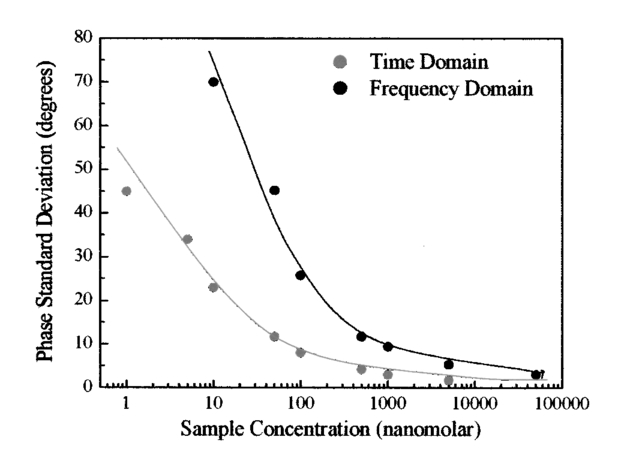

To provide an example of what to expect in a typical microscope experiment, we show in Fig. 6 the histogram of phase values calculated after fast Fourier transformation from TCSPC data acquired with a pixel residence time of 1 ms for the 1-μM fluorescein solution using our two photon microscope. The total counts collected for each decay determination was about 1000 per pixel. The standard deviation of the phase measurement is a about 2.4 deg, which corresponds at 80 MHZ to 0.4 ns.

Figure 6

Phase standard deviation from the time-domain data of an image (256×256) for a 1-μM fluorescein solution. The absolute phase value has not been referenced to the reference compound.

Table 3 shows the harmonic analysis of the FFT time-domain data averaging 4 neighbors pixels selected in a region of the image. As expected, only a few harmonic components can be reliably used at this count level. We performed a fit of this frequency-domain-translated decay using the Globals WE software. The recovered average lifetime is 4.1±0.7 ns and the residues were very large. A similar result is obtained if we perform the fit directly in the time domain.

Table 3

7.

FLI of Cells Expressing EGFP

In this section, we report first FLI of YFP’s constructs with the PAT4 protein in the muscle of C elegans. This sample was provided by Dr. B. Williams of University of Illinois. On the same worm, we performed time-domain and frequency-domain measurements. Although the laser conditions are the same, the image area is not identical in the two examples. In this study, the image intensity is very low and we should be in the low counting regime discussed in the previous sections. Figure 7 (see Color Plate 1) shows the TCSPC FLI image obtained with the B&H630 card. The pixel time for this image was 1 ms obtained by averaging 10 frames with a pixel time of 100 μs. The instantaneous maximum counts per pixel (about 40,000 counts/s) should always be below the saturation limit of the card. Only pixels with at least 30 counts were analyzed. Pixels were not averaged together. The FLI images are presented in terms of τ_ϕ and τ_m, according to the discussion in the previous section. The lifetime is relatively homogeneous across the image, although the intensity varies from 30 counts (minimum) to about 400 counts (maximum). The histogram of lifetime values are centered at 2.7 and 3.5 ns for the phase and modulation determination, respectively. This is expected since in a nonhomogeneous system, the phase lifetime is always less that the modulation lifetime. The standard deviation of the lifetime determination is about 1 ns, as expected from the photon statistics of about 100 counts per decay curve.

Figure 7

Time-domain FLI images of YGFP in C. elegans PAT4 construct. The tau phase and tau mod images were calculated using the formulas in the text and if the intensity value was above 30 counts in the pixel.

The frequency-domain FLI measurements are shown in Fig. 8 (see Color Plate 1). The values in Fig. 8 are comparable to the values in Fig. 7. The integration time per pixel was 0.8 ms for Fig. 8. For the FLI analysis, only points with at least 2 nA were analyzed. The average lifetime histograms are comparable with those of Fig. 7. However, the relative standard deviations of the lifetime histogram is larger for the frequency-domain determination, in accord of the smaller SNR of the frequency-domain measurements in the low-counting regime.

Figure 8

Frequency-domain FLI images of YGFP in C. elegans PAT4 construct. The tau phase and tau mod images were calculated using the formulas in the text and if the photocurrent value exceeds 2 nA in the pixel. Color Plate 1

Next, in Fig. 9 (see Color Plate 2) we show FLI images of the construct AK-EGFP in HeLa cells. Left is the intensity image and right is the phase image. The image was obtained at a rate of 100 μs/pixel. Intensity and phase histograms from a region of about 4600 points in the interior of the cell are also shown in the bottom part of the figure. In this case, the intensity histogram in the frequency domain is centered at about 1000 nA. The intensity expressed in current is independent on the pixel residence time. Using the curves of Fig. 4 an from which we derive that 1 nA is approximately 10,000 counts, our estimate of the equivalent instantaneous counting rate per pixel is about 10⁷ photons/s for the bright spots of this image. Note that the counting rate for this image is well above the upper limit permitted by our TCSPC card. The effective number of photons detected in 100 μs for the bright spots is about 1000. The phase histogram shows a standard deviation of approximately 5 deg which, translated to lifetime (at 80 MHZ), corresponds to about 0.7 ns.

Figure 9

Frequency-domain FLI images of AK-EGFP in HeLa cells. Phase and intensity histograms are for the square-region in the screen.

8.

Discussion

Figure 10 (see Color Plate 2) schematically shows the different ranges of operation for the two fluorescence lifetime measurement methods. The green region, which is the region of operation of the TCSPC electronic, is drawn assuming that at most 10⁶ counts can be processed per second. This is at the limit of our particular electronics (B&H model 630 card). We note that faster electronics are now available. Our only purpose is to show that there is a limit of counts above which the TCSPC detection will saturate.

Figure 10

Lifetime map plot showing regions in which each technique could be applied. For a discussion of this figure see the text. Color Plate 2

In a log-log plot the differences between different acquisition electronics and manufacturers give lines that are almost one on top of one another. For the frequency-domain method, this boundary line due to the recovery time for the card does not exist. Another important line in this figure is the time for pixel acquisition. We choose as a limit 400 μs/pixel that gives about 26 s for frame acquisition for a 256×256 image. This limit is arbitrary, since in principle the time spent in a pixel can be made longer. However, in our experience using living cells, 26 s is considered an upper limit. The frame size can also be reduced at the expenses of either image resolution or field of view. Again, the graph of Fig. 10 should serve only as a reference. Another important family of lines is the number of molecules per pixel. The number of molecules is estimated using fluorescein as an example and assuming that one molecule of fluorescein produces about 30,000 counts/s. Of course, this figure depends on the microscope setup, the laser intensity, and other instrumental parameters. Using this estimation, the graph shows that above about 30 to 40 molecules/pixel, the TCSPC method cannot keep up unless the average laser intensity is reduced. In practice, what is usually done when using the TCSPC method is to reduce the laser repetition rate. Instead of operating the laser at a high repetition rate (generally 80 MHz), the laser frequency is divided by a factor (generally 10 or 20) using a pulse picker or a cavity dumper. Apparently, there is very little penalty in performing this operation in the context of the TCSPC method, since the acquisition rate in the TCSPC method is determined by the speed of the electronics. In fact, most TCSPC systems operate either at 4 MHz laser frequency or less. When comparing the time-domain and the frequency-domain methods, the same amount of photons detected can be obtained during a much smaller integration time in the frequency domain operating at 80 MHz since the detector does not saturate. This is crucial for the microscope environment where the total duration time of frame acquisition cannot be very large. If the number of fluorophores per pixel is below 30, then the TCSPC method can process all the data, and in this regime, the time-domain method provides a better SNR.

Another useful set of lines in this figure is the family of lines for the required counts to resolve multiple components. In our estimates, we determined that we need at least 100 counts in the histogram to obtain a lifetime with an uncertainty of about 20. To resolve two components, under ideal circumstances, i.e., when the lifetimes of the components are well separated and the two components have comparable intensity, we require about 1000 photons to resolve the system. For 3 components, we require a factor of 10 more. These are only order of magnitude estimations and the actual number of counts required varies depending on the separation and relative intensity of the lifetime components. In normal practice for TCSPC measurements in a cuvette, much larger numbers of counts are collected in a decay curve because a better precision in the resolution of multiple components is the goal for cuvette measurement. Inspection of Fig. 8 shows that the TCSPC method could separate two components in the microscope environment only for very long frame integration times. In fact, the region in cyan color in the figure is the region in which the TCSPC method could be used in the microscope. Clearly, this is a small region of the counts per pixel time space. In many situations in microscopy, we are dealing with 100 or 1000 molecules in a pixel. This region cannot be reached with short integration times using the TCSPC method. The laser repetition rate or the laser intensity must be attenuated to fulfill the counting rate requirements of the TCSPC electronics. The frequency-domain technique is not limited by a high count rate.

9.

Conclusions

In principle, the SPC electronics provides a better SNR because of the discrimination of the dark counts and because of the assignment of a specific delay to each photon. For very weak fluorescent samples and using long integration times, this capability could be advantageous. However, this advantage is not crucial if we consider that the frequency-domain method is intrinsically based on a lock-in method and that the dark noise is also very efficiently discriminated.

For the microscope environment, the potential advantage of the TCSPC method is reduced by the relatively slow processing electronics. We have estimated that in common experiments, the rate of photon detection in the bright pixels in a typical image is well above the processing capability of the SPC electronics. This effect results in fewer photons detected, distortion of the image intensity, and overall increase of the noise. Our conclusion is that the TCSPC method is advantageous for weak samples and using very long integration times. For example, for single molecule studies it is the only possibility. In all other conditions, the analog frequency-domain method could result in an overall better SNR due to the smaller dead time and to the lack of saturation of the detection electronics.