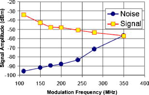
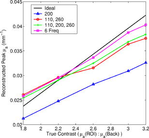
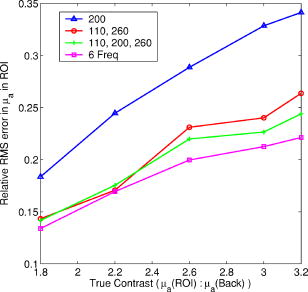
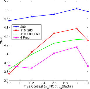
1.

Introduction

There has been great interest in the field of near-infrared (NIR) imaging in the last two decades. ^{1, 2, 3, 4, 5, 6, 7} The fundamental reasons behind this interest are the ability of the optical imaging systems in providing chromophore-related information such as oxy-hemoglobin $\left(\mathrm{HbO}\right)$ , deoxy-hemoglobin (Hb), fat, water content, and scattering-related information, such as scatterer density and scatterer size within the biological tissue. Hemoglobin concentration has been used as a tool for functional imaging of human cerebral activity and cancer detection based on the associated vascularity. ^{8, 9, 10, 11, 12, 13} Meanwhile, scattering parameters provide the information about the differences in cellular and organelle density, and size within the tissue.¹⁴

Diffuse optical tomography (DOT) is a recently emerging optical imaging technique that uses arrays of sources and detectors to obtain spatially dependent optical parameters of tissue. The steady-state (continuous wave, CW), the time-domain (TD), and the frequency-domain (FD) diffuse optical tomography methods are the main techniques developed for quantification and spatial localization of variations in tissue.¹ CW systems provide only magnitude information and do not allow an effective way to distinguish between the effects of absorption and scattering.¹⁵ In the time domain, a laser pulse is sent to the tissue and the delay of the light is measured to estimate the absorption inside the tissue. The time-domain systems measure the temporal distribution of photons produced when a pulse of light is transmitted through the medium. The information content in a temporal point spread function (TPSF) is more than frequency-domain measurements consisting of phase and amplitude measurements at a certain modulation frequency.¹ The intensity and mean photon flight time calculated from the TPSF are almost equivalent to the amplitude and phase of a frequency-domain system.¹⁶ However, the frequency content of the TPSF extends to several GHz. On the contrary, diffuse optical tomography techniques generally use a single modulation frequency due to the complexity of the instrumentation and time limitations. In our previous work, we presented the development of a multifrequency DOT instrumentation.¹⁷

In this study, we investigate the performance of our multifrequency reconstruction scheme as a function of the number of modulation frequencies. Although the information content of such a multifrequency scheme will always be less than the information content in a TPSF, this study is an attempt to increase and optimize the efficiency of the frequency-domain DOT, which is an easier and cheaper alternative to the time-domain DOT.

While light propagates through the tissue, it is absorbed by the chromophores. Although the absorption information is sufficient to find the chromophore concentrations, the scattering map must also be reconstructed simultaneously due to the cross-talk in measurements of the optical parameters. Separation of absorption and scattering is required for quantitative imaging of these chromophores. It has been found that higher modulation frequencies give a better separation of absorption and scattering properties.¹⁸ The accuracy of phase measurements limits the quality of images, especially in the case of small objects where the shift in phase is low. As the frequency increases, the phase shift difference between normal and tumor tissue increases.¹⁹ Therefore, higher frequencies provide a better detection of small objects.¹⁸ However, since the signal-to-noise ratio (SNR) decreases with the increasing frequency as shown in Fig. 1 , the sensitivity and accuracy of the detection system decrease.¹⁹ It was experimentally shown that the image quality depends on the modulation frequency, and an optimum frequency exists depending on the SNR of the system in amplitude and phase at different frequencies.¹⁷

Fig. 1

The dependence of signal and noise on the modulation frequency.

At this point it is clear that both high- and low-modulation frequencies have certain advantages and disadvantages. It is well accepted that the image quality and accuracy of reconstructed optical parameters are both issues of important concern in optical imaging. In this study, we present a technique where we employ the multifrequency data simultaneously in the reconstruction.¹⁷ This approach combines the advantages of low-frequency and high-frequency modulation and improves the image quality and accuracy of the reconstructed optical parameters. A multiparameter Tikhonov method was applied for the regularization. The quality of the reconstructed images using different combinations of modulation frequency data was investigated. We used a Newton-type algorithm to obtain the solution that minimizes the error between the measured data and the estimated measurements from the forward solver. A fan-beam detection geometry was used and a fiber optic interface was constructed. Solid-liquid phantoms were used to evaluate the performance of the system. The results showed that the multifrequency reconstruction improves the image accuracy and quality. The results also indicated that the use of two frequencies for the reconstruction is adequate to obtain a significant improvement. This is an important factor in achieving a reasonable data acquisition time, especially required for clinical studies.

Several groups working in the frequency domain have already suggested the possibility of improving DOT reconstruction using multifrequency data. A modulation-frequency-dependent improvement in resolution is expected when the background absorption is low enough so that the resulting phase shift has a strong dependence on the modulation frequency.²⁰ Milstein present a Bayesian DOT reconstruction algorithm to investigate the benefits of using multiple modulation frequencies in DOT²¹ and fluorescence DOT.²² They showed that the simultaneous use of multifrequency data with a priori information in the reconstruction improves the image quality in some cases. Gao ²³ showed that image quality is improved in DOT by the use of full time-resolved data. This paper is different from these previous studies, which concentrate on the resolution, in that we show that the accuracy of the optical parameters can be improved using the multifrequency reconstruction. In addition, we discuss the selection of the optimum frequencies and the use of multiparameter Tikhonov regularization. We present the first detailed experimental analysis on the use of multiple modulation frequency data in frequency-domain DOT.

In the next section, we review the diffusion equation and explain the simultaneous use of the multifrequency data in reconstruction. In Sections 3, 4, we present the experimental setup and the results, respectively.

2.

Numerical Modeling

3.

Experimental Setup

In order to test the multifrequency reconstruction, we carried out a series of phantom experiments using our MF-DOT system. The details of the instrumentation are given in the paper by Gulsen ¹⁷ In this section, we briefly discuss the key components of the instrumentation and the phantom experiments.

The MF-DOT system is based on a network analyzer. The network analyzer not only provides the radio frequency (rf) signal to modulate the amplitude of the laser diode sources, but also measures the amplitude and the phase of the detected signals. The system employs four different wavelengths, namely $665\mathrm{nm}$ , $785\mathrm{nm}$ , $800\mathrm{nm}$ , and $830\mathrm{nm}$ . We used 7 different modulation frequencies: $110\mathrm{MHz}$ , $140\mathrm{MHz}$ , $170\mathrm{MHz}$ , $200\mathrm{MHz}$ , $230\mathrm{MHz}$ , $260\mathrm{MHz}$ , and $280\mathrm{MHz}$ . The maximum modulation frequency was chosen in accordance with the system’s SNR limitation.¹⁷ The selection of the wavelength, $785\mathrm{nm}$ , was arbitrary.

Photomultiplier tubes (PMT) were used as detectors. As we mentioned previously, the SNR in amplitude decreases with increasing modulation frequency because of the limited bandwith of the PMT. Therefore, the performance of the MF-DOT system is closely related to the performance of the PMTs.¹⁷ The average noise level of the system was around $-90\mathrm{dBm}$ up to $200\mathrm{MHz}$ , $-80\mathrm{dBm}$ up to $250\mathrm{MHz}$ , $-70\mathrm{dBm}$ up to $300\mathrm{MHz}$ , and $-55\mathrm{dBm}$ up to $350\mathrm{MHz}$ . The bandwidth of the system is selected as the frequency at which the SNR drops below $10\mathrm{dB}$ ; it is determined as $280\mathrm{MHz}$ (Fig. 1). The minimum detectable signal at this frequency is $-67\mathrm{dBm}$ , which corresponds to light power of $0.4\mathrm{pW}$ incident on the detector.

Two 63-mm-diameter solid phantoms simulating tissue optical properties were constructed using the method described by Firbank ³⁰ These phantoms were constructed for the small animal imaging purposes. Therefore, the optical parameters of the phantoms were adjusted accordingly ( ${\mu }_a=0.013{\mathrm{mm}}^{-1}$ and ${\mu }_s^{\prime }=0.858{\mathrm{mm}}^{-1}$ at $785\mathrm{nm}$ ). One of them was used for calibration purposes (homogeneous case), and a 15-mm hole was drilled in the other one between the center and the edge as shown in Fig. 2 . The simulation of different embedded objects (heterogeneous case) was performed by filling the hole with varying concentrations of Intralipid (10%) and Indian ink in water. Solutions with contrast ratios of 1.8:1, 2.2:1, 2.6:1, 3.0:1, 3.2:1 in absorption with respect to the phantom absorption coefficient were prepared. The data were obtained at seven modulation frequencies. The MF-DOT system consists of 8 sources and 8 detectors and is fully automated. In our system, the acquisition time for a full tomographic scan of 64 complex data points at a single wavelength and single modulation frequency is around $220\sec$ . Data acquisition times for two, three, and six frequencies are around $380\sec$ , $480\sec$ , and $840\sec$ , respectively.

Fig. 2

The phantom with a 15-mm hole inside.

Calibration is the pivotal part of the data acquisition due to the variation in characteristics of each PMT, optical fiber, and neutral density filters. The calibration procedure for our DOT system was given in detail previously.¹⁷ An accurate calibration is achieved in three steps: filter calibration, detector calibration, and homogeneous phantom calibration.

The filter calibration is done to find the optical density (OD) of each individual filter at different positions. The filter OD values are recorded to a calibration file to calibrate all the data obtained from a measurement set. The detector calibration is done by placing a source at the center of the phantom and recording the measurements at each detector site. Each detection fiber is exposed to the same optical signal, and the differences in the amplitude and phase measurements are recorded as calibration factors. This calibration step identifies the differences of the detector fiber-PMT combinations and the performance of the corresponding rf switch ports that determine the signal strength measured from detection sites.^{30, 31}

A complete set of measurements from a homogeneous phantom is used for the last calibration step. This calibration is performed to account for the fiber differences in transmission and alignment and the discretization errors due to data/model mismatch.³¹

Measurement repeatability is also an important factor that affects the performance of the imaging system. To separate the errors arising from the fiber positioning and the instrument itself, we conducted repeatability tests with and without the repositioning of the homogeneous phantom.³² First, the phantom was placed in the fiber optic interface and measurements were repeated 10 times. The average rms errors in the amplitude and phase measurements were found to be 0.5% and 0.2°. The repeated measurements were also acquired for the case in which the phantom is removed and repositioned between each measurement. To eliminate the errors due to the phantom’s inhomogeneity, the phantom was placed in the same orientation each time it was repositioned. In this case, the average rms error in the amplitude and phase measurements were found to be 5% and 0.4°. This error was caused only by the fiber probe repositioning.

4.

Results

In this section, we present the results of the phantom experiments. We compare the reconstruction results of the single-frequency and multifrequency data. First, the parameters used to evaluate the quality of reconstructed images are defined. Next, the results for single- and multifrequency cases are presented.

4.2.

Comparison of Single-Frequency and Multifrequency Reconstructions

We investigated the performance of the reconstruction using the parameters defined in Section 4.1. We compared the $200\mathrm{MHz}$ results with several multifrequency reconstruction results since the $200\mathrm{MHz}$ was shown to be the optimum frequency for our imaging system.¹⁷ We investigated the performance of the use of two and three frequencies in the reconstruction as well as the performance of the use of the six frequencies. Although a number of different combinations of multifrequency data were used in reconstructions, we only present $110–260\mathrm{MHZ}$ , $110–200–260\mathrm{MHz}$ , and 6-frequency results. The presented combinations provide the best results. Note that we do not use the $280\mathrm{MHz}$ data since the noise level at this frequency suppresses the advantages of the two- or three-frequency reconstruction. We discuss this in more detail in the next section.

Figure 3 shows the graph of the reconstructed peak ${\mu }_a$ in ROI versus different contrast levels. The results are plotted for single- and multifrequency reconstructions and compared with the true peak values. The error in the reconstructed peak ${\mu }_a$ increases with the increasing contrast level as expected. An important observation is that the multifrequency reconstruction becomes more effective with the increasing contrast level and recovers the absorption coefficient with less error. For example, for the contrast ratio of 3.2:1 $({\mu }_a=0.042{\mathrm{mm}}^{-1})$ , the peak absorption value recovered by 6-frequency reconstruction was $0.039{\mathrm{mm}}^{-1}$ , while the value recovered by single-frequency reconstruction was $0.032{\mathrm{mm}}^{-1}$ . Likewise, the use of two frequencies, 110 and $260\mathrm{MHz}$ , or three frequencies, 110, 200, and $260\mathrm{MHz}$ , still gives significantly improved peak values, $0.036{\mathrm{mm}}^{-1}$ and $0.0365{\mathrm{mm}}^{-1}$ , respectively. Note that the use of a smaller number of modulation frequencies is important in order to reduce the data acquisition time to make such measurements practical for in vivo studies.

Fig. 3

Reconstructed peak ${\mu }_a$ versus contrast ratio of ${\mu }_a$ with respect to the background.

Figure 4 illustrates the rms error in ROI versus different contrast levels. The figure shows that the rms error increases with the increasing contrast level as expected. The improvement in the accuracy significantly increases by the use of multifrequency data in each contrast level. Furthermore, it is also evident that the performance of the two-frequency $(110–260\mathrm{MHz})$ reconstruction is sufficient to obtain a considerably accurate absorption coefficient value in ROI. Figure 5 plots the CNR versus different contrast ratios. The highest CNR values are observed in the results for $200\mathrm{MHz}$ . This was expected since the data at $200\mathrm{MHz}$ are less noisy compared to the data obtained from combinations of 110 and $260\mathrm{MHz}$ , or 110, 200, and $260\mathrm{MHz}$ , or all six frequencies.

Fig. 4

Rms error in the ROI versus contrast ratio of ${\mu }_a$ with respect to the background.

Fig. 5

CNR versus contrast ratio of ${\mu }_a$ with respect to the background.

Figure 6 shows the IC values for different contrast levels. From the definition in Eq. 14, it is evident that the IC increases as the image quality improves and the accuracy of the recovered optical parameters increases. Figure 6 shows that the IC obtained using the multifrequency data is higher than the single-frequency counterpart. Figure 7 illustrates the reconstructed ${\mu }_a$ and ${\mu }_s^{\prime }$ maps for the contrast levels 1.8:1, 2.6:1, and 3.2:1. It is observed that the use of more than two frequencies does not improve the image quality significantly; on the contrary, the scattering maps become more noisy.

Fig. 6

IC versus contrast ratio of ${\mu }_a$ with respect to the background.

Fig. 7

Reconstructed ${\mu }_a$ and ${\mu }_s^{\prime }$ images for 1.8:1, 2.6:1, and 3.2:1 contrast ratio.

These results demonstrate that although utilization of two-frequency data in the reconstruction is adequate, for high contrast levels, the use of more than two frequencies gives more accurate results for an ROI at the expense of reduced CNR and increased background noise.

5.

Discussion

The rationale of optical imaging has been based on only endogenous differences in the absorption and/or scattering properties between the normal and diseased tissues. The endogenous contrast arises due to different hemoglobin content and scattering properties of the tumor. For example, images of breast lesions indicate that total hemoglobin-based contrast can be up to 2 times higher relative to the background in the same breast. However, the optical imaging field has been rapidly expanding in scope through the use of new exogenous molecular probes. Some of these new exogenous probes can increase the contrast further by a factor of two or more. Therefore, we have chosen an absorption contrast of 1.8 to 3.2 in our studies.

The set of appropriate frequencies for the reconstruction is determined mostly by the SNR properties of the imaging system at different frequencies. The use of multifrequency data is expected to improve the reconstruction since there are more singular values over the noise level compared to the single-frequency case. While the use of 110 and $260\mathrm{MHz}$ gives a significant improvement in the image quality, the use of 110 and $280\mathrm{MHz}$ does not because the noise in $280\mathrm{MHz}$ data is higher than the $260\mathrm{MHz}$ data. On the other hand, the $110–260\mathrm{MHz}$ reconstruction gives much better results than the $110–140\mathrm{MHz}$ one since the information content is more distinct in the $110–260\mathrm{MHz}$ combination. Figure 8 shows the raw data obtained at 110, 260, and $280\mathrm{MHz}$ . As the figure shows, the amplitudes measured by 64 detectors are distributed in a certain range. The difference in the measurements arises from the different photon path traveled for different source detector pairs as well as the position of the object. This range is still very small compared to the dynamic range of the real light distribution collected by the fibers due to the filters used to reduce the dynamic range of the optical signal. As seen in Fig. 1, the SNR in amplitude decreases with the increased frequency due to a decrease in the signal amplitude and an increase in the noise level. For instance, for this particular source-detector pair that provides the lowest signal, the SNR in amplitude reduces approximately from $30\mathrm{dB}$ down to $10\mathrm{dB}$ as the modulation frequency increases from $110\mathrm{MHz}$ to $280\mathrm{MHz}$ . Meanwhile, the SNR in the phase increases due to not only an increase in the measured phase shift but also the constant phase noise of network analyzer. Although the network analyzer keeps the phase error constant as the signal amplitudes decrease, when the signals drop below $-50\mathrm{dBm}$ , the error in the phase measurement starts increasing. Therefore, $-50\mathrm{dBm}$ is an important threshold for our measurements beyond which the SNR in phase starts to decrease. As the modulation frequency increased, more and more measurements that belong to the farthest source-detector pairs drop below $-50\mathrm{dBm}$ . Indeed, Fig. 8 shows that there is a three-fold increase in the number of the measurements below $-50\mathrm{dBm}$ , from 4 to 11, as the frequency increases from 260 to $280\mathrm{MHz}$ . This is the main reason that the data acquired at $260\mathrm{MHz}$ give more accurate reconstruction than the data acquired at $280\mathrm{MHz}$ .

Fig. 8

The raw data obtained at 110, 260, and $280\mathrm{MHz}$ .

In general, for an optical tomography system with fan-beam geometry, the measurements from different source-detector pairs will be different. To be able to select the proper modulation frequencies, the dynamic range of the signals should be determined and the SNR in amplitude and phase should be characterized as a function of frequency for that particular system. The lowest amplitude value should be determined beyond which the phase error of the detection unit increases. The highest modulation frequency that could provide the measurements above that lowest amplitude should be selected as maximum modulation frequency of the system. Once the maximum modulation frequency that provides the highest phase SNR is determined, this maximum frequency can be used along with the lowest modulation frequency that provides the highest amplitude SNR for the multifrequency reconstruction. The most common modulation frequency for the DOT systems is $100\mathrm{MHz}$ ; this value can be chosen as the minimum frequency.

Although the utilization of two carefully selected modulation frequencies improves the image accuracy, the accuracy can further be improved by using a greater number of modulation frequencies in the analysis, especially for higher contrasts. For instance, for the absorption contrast of 3.2, the error in the reconstructed absorption peak reduced from 22% to 3% when six different modulation frequencies were used instead of two. On the other hand, the noise in the background in scattering and absorption maps increased in parallel to the increasing number of modulation frequencies used in the reconstruction, and as a result CNR decreased and the image quality was not improved significantly. Further investigation of the use of multifrequency data in highly heterogenous medium is required.

6.

Conclusions

In this paper we present results employing simultaneous reconstruction of multiple modulation frequency data for diffuse optical tomography. We investigate the contrast-to-noise ratio, the peak absorption coefficient in the region of interest, the root mean error in the region of interest, and the image coefficient. The results show that multifrequency reconstruction yields improved quantitative accuracy in absorption maps compared to the single-frequency reconstruction. Since the accuracy of the optical parameters is very important for the clinical applications of DOT, this novel approach is expected to be very useful in tumor monitoring by means of optical imaging.

Moreover, the results showed that by proper selection of modulation frequencies, even the two-frequency data set will improve the reconstruction quality and accuracy compared to the single-frequency reconstruction. These two modulation frequencies must be chosen with respect to the SNR levels in amplitude and phase of the imaging system. Therefore, this selection would be different for different imaging systems. Of course, the utilization of only two modulation frequencies will reduce the data acquisition time compared with greater frequency cases; therefore, it is important for clinical and even dynamic optical imaging studies.

This study was an attempt to increase and optimize the information content of the frequency-domain DOT, which is an easier and cheaper alternative to time-domain DOT. The frequency range was determined by the minimum and the maximum frequencies, as explained in Section 5.

Combined imaging systems such as MRI or CT, which provide the structural information along with the diffuse optical tomography, make it possible to choose a region of interest (ROI) within the tissue to be imaged. Therefore, the peak and rms values of the optical parameters within the ROI become important. The results demonstrated that the multifrequency reconstruction reduces the error in the peak and rms values of the absorption coefficient. Indeed, if one is only interested in recovering the absorption in ROI for high-contrast levels, it might be beneficial to use more than two modulation frequencies for the reconstruction.

It is also expected that the direct chromophore reconstruction can be improved by the use of multifrequency data. It has been shown that the error in the reconstructed absorption coefficient for an inclusion in the tissue results in a higher error in the chromophore reconstruction, e.g., water content in the breast.³⁴ The accuracy of chromophore reconstruction is vital for the potential clinical applications of diffuse optical tomography. Multifrequency reconstruction would provide this accuracy when combined with the multiwavelength reconstruction. We are going to investigate this issue in our future work, studying the multifrequency, multiwavelength reconstruction results for the conventional chromophore and direct chromophore quantification.