
|
|
1.IntroductionFlow and image cytometers are instruments that measure cells and are in wide use in clinical and research settings. Flow cytometers, which began in the 1950s with the Coulter counter and attained fluorimetry capabilities in the 1960s,1 are much more prevalent because of advantages in speed and automation, despite the superior information content of 2-D images relative to 1-D flow data. Commercial flow cytometers can reach ,2 while image cytometers typically process cells at under at moderate magnification/resolution.3 Speeds of more than have been reported in imaging4 at low magnification where depths of field are large and autofocus performance is not critical. Although image cytometers have recently achieved the same level of walk-away automation for large cell populations3 [see also high content screening instruments from Beckman Coulter (Fullerton, California), Cellomics (Thermo Fisher Scientific, Pittsburgh, Pennsylvania), GE-Amersham (Buckinghamshire, United Kingdom), Evotec Technologies (Hamburg, Germany), BD Biosciences (Boston, Massachusetts), Molecular Devices Corporation (Sunnyvale, California), and the Compucyte Corporation (Cambridge, Massachusetts)], experience with flow cytometry and the demands of applications in fields like clinical diagnostics and drug discovery suggest that image cytometry use may expand dramatically with similarly high throughput. Throughputs an order of magnitude greater can be achieved by moving the sample in a continuous motion.5, 6 But robust autofocus performance in high-resolution optical microscopy, where depths of field are on the order of , has been challenging7, 8 and has not previously achieved the performance required for widespread use of continuous-scanning image cytometry. The two primary approaches to autofocus are: 1. position sensing, usually based on light reflection off of the specimen surface substrates,9, 10, 11 and 2. image content sharpness measurements, wherein the image quality is maximized directly to achieve best focus. 7, 8, 12, 13, 14 Surface sensing is best for total internal reflect fluorescence (TIRF) microscopy, because the position of the focal plane directly adjacent to the surface is fundamental to the physics of fluorescence generation (e.g., the Nikon Perfect Focus System). It is also widely used for lower resolution, large depth of field image cytometry. Image-content-based autofocus works best for medium- and high-resolution automated microscopy , where the depths of field approach or become even smaller than the thickness of the tissues and where the specimens vary in height and thickness. The drive to use higher NA objectives arises from the need to improve resolution, which is a function of NA, and increase fluorescence light gathering power, which is a function of .15 The dependence of fluorescence light gathering is particularly dramatic and in many cases may explain, even more than the increase in resolution, why tiny details become so much more visible in fluorescence as NA is increased. Since depth of field is a function of ,15 autofocus challenges increase substantially with NA. These challenges and tradeoffs have made autofocus an active microscopy research topic for many years. Here we report adapting our image-content-based autofocus methods to create dynamic image-content-based autofocus for medium- and high-resolution continuous scanning. The system parallelizes our previous autofocus methods to image and measure the sharpness of multiple focal planes in parallel for on-the-fly autofocus. For use in a wide range of applications, a high-performance image cytometer should acquire and process large quantities of data at submicron resolution, e.g., about 20,000 1-Mpixel images for an area of one microscope slide at /pixel sampling [with a resolution objective (Rayleigh, and ) and a CCD camera Nyquist sampling , the field of view is and 19,868 images are needed to cover the area of a microscope slide]. Conventionally, the cells are scanned by moving a stage between each field of view (FOV) and stopping to autofocus and capture an image.3 Good autofocus is fundamental to the quality of a microscope image in an automated instrument; the quality of the measurements and observations drawn from the image are dependent on sharp focus. Autofocus is perhaps even more important in automated image cytometry, because image segmentation (as well as other image processing and analysis operations) and the resulting measurements are sensitive to focus. Autofocus is critical for maintaining consistent image sharpness because slides, coverslips, and plates are far from flat (relative to the depth of field), and mechanical instabilities that include thermal expansion, gear backlash, and settling are best countered by corrective feedback. In lower resolution systems, autofocus is sometimes performed on only every five or ten fields to increase speed. For NAs of 0.5 or more where depths of field approach or less, however, measurement precision can be compromised by infrequent autofocus. Here, we report our exploration of parallel multiplanar image sharpness measurements for continuous autofocus to overcome the speed limitations of our current systems, in which the repeated acceleration and deceleration of a relatively massive stage to sequentially image many adjacent fields of view fundamentally limits speed. We found that acceleration-induced vibration that degrades imaging and autofocus performance can be easily achieved with the commercial motorized stages routinely used in microscopy. Sequential stage motion, autofocus, and image capture are also inefficient simply because the camera is not acquiring an image for cytometry during autofocus and stage movement. Previous designs for moving the stage continuously to overcome these problems and increase speed are summarized in Table 1 . The system by Netten 16 followed a prerecorded focus path during continuous scanning, as does the Aperio Technologies (Vista, California) brightfield system for scanning tissue sections. The system by Castleman17 apparently paused to perform static autofocus at regular intervals, and those by Shippey 18 and Tucker 19, 20 autofocused dynamically during scanning. Both Shippey 18 and Netten 16 reported that the focus error was greater than the depth of field, and Tucker 19 reported that a focus error produced a 12% error in the integrated optical density of the cell nucleus. Autofocus accuracy was reported to be very dependent on the density of cells by Castleman,17 and the need for many cells in each field of view was common to all of the systems that included autofocus. None of these designs have been widely adopted. The techniques and problems reported with them in these studies point to limitations in automatic operation, large focus errors that would limit use in high-resolution microscopy, relatively few focus updates per image field, and too much dependence on cell density for reliable focus tracking, perhaps due to limited sharpness measurement sensitivity and dynamic range. Table 1Previously reported continuous-scanning instruments. AF autofocus, NR denotes not reported in listed reference, IOD is integrated optical density, and CV is the coefficient of variance.
More recently, the GE-Amersham (Buckinghamshire, United Kingdom) In Cell Analyzer 3000, which uses reflection positioning off of the surface of the substrate for focusing a laser slit-illuminated partial confocal light beam that is scanned continuously, was introduced for high content screening. The partial confocal imaging corrects for medium resolution focus errors by removing some out-of-focus image information to perform optical sectioning, which makes it less critical to find the average best focus across the field. Similarly, the Evotec Opera (Woburn, Massachusetts) and the Atto Pathway HTTM system use spinning disk confocal image acquisition to remove out-of-focus light. These confocal systems tend to be 2- to 3-fold more expensive than wide field fluorescence instruments. These and most other automated microscope manufacturers have not published autofocus performance. To maximize light collection efficiency and begin with the simplest optics, we chose to base the system reported here on wide-field fluorescence imaging. Because thermal and mechanical instability can cause focus to change between scans of the same area, and prescan focus profiling can be time consuming for high-resolution images, we also assumed that dynamic autofocus during scanning is a requirement for high fidelity and ease of use. With high-resolution scanning , measurement accuracy degrades if autofocus is not performed on each field of view. The designs by Shippey 18 and Tucker 19, 20 that included dynamic autofocusing sampled only two focus planes and utilized integrated optical density (IOD) for measuring focus. Static (fixed lateral position) image-content-based autofocus experiments have shown that 7 to 11 planes are usually required for robust autofocus, that intensity statistics (e.g., mean, or IOD, and SD) are poor measures of focus 7, 8, 12, 13 and that the power of the upper-half spatial frequency image spectrum as a measure of sharpness is the best measure of focus.14 We therefore combined this sharpness measurement with multiplanar image acquisition to build and test on-the-fly continuous-scanning closed-loop autofocus. Concurrent with the task of high-resolution autofocus, the use of continuous-motion time-delay-and-integrate (TDI) scanning has the potential to dramatically speed image acquisition while retaining high light sensitivity. TDI scanning is a special CCD readout mode that increases the integration period by allowing multiexposure of a moving object when its motion is synchronized to the CCD line rate, producing a 2-D image. A TDI CCD has multiple adjacent linear stages (e.g., 96), that transfer and integrate the photo-generated charge from line to line synchronously with the motion of the imaged object, increasing sensitivity (e.g., 80 times for 96 stages) over a single line array. This method has been adopted in our image cytometer to increase sensitivity in fast image acquisition, and we have developed a dynamic autofocus system that maintains spatial high resolution by tracking focus during the microscope stage motion. A continuously moving object can be imaged by strobed lighting or by synchronizing a linear CCD with the motion. Because fluorescence saturation fundamentally limits the amount of light per unit time that can be obtained from the specimen, we incorporated TDI cameras, which increase photosensitivity by increasing the integration time proportional to the number of CCD lines. TDI sensors are often used in machine vision applications to detect and identify defects on continuously moving objects (e.g., manufactured parts on an assembly line). For web inspection, the object in the field of view of the sensor can be assumed to be flat because the depths of field of macroscopic optics are usually large, enabling focus to be adjusted to include the extent of the object.21 In these applications, resolution (which drives higher NAs/lower F-stops that reduce depths of field) is not usually a limiting factor. Where depths of field are limited, the autofocus technique described here may also be useful for web inspection. For any TDI application, proper synchronization of image acquisition with motion is required to avoid blurring and maintain proper horizontal to vertical aspect ratios in the acquired image (i.e., square pixels). TDI technology has also been applied to create an imaging flow cytometer with high resolution and fluorescence sensitivity at speeds of up to .22, 23, 24 The advantage in flow cytometry is that hydrodynamic focusing can be used to keep the cells in the focal plane. The image acquisition is synchronized to the fluid flow for TDI imaging.25 With cells flowing in a single file, the additional lateral area on the TDI CCD is utilized for additional analyses, including spectral imaging and 3-D structure.24, 26, 27 Autofocus is performed by moving the objective in response to a difference signal generated by two detectors sensing light modulated by two Ronchi rulings deployed behind a 50/50 beamsplitter.28 It is not known if this autofocus method would work for image cytometry, but other intensity-based autofocus methods have not performed well for microscopy of specimens on a substrate.12 Based on our experience with static autofocus 7, 8, 14, 29 in automated microscopy of specimens on substrates, we developed and tested dynamic autofocus for a continuous-scanning system. Our static image-content-based techniques were converted to dynamic autofocus by designing an electro-optical system for acquiring multiple image planes at predetermined focal depths in parallel, which we named the “volume camera.” The volume camera also uses TDI CCD sensors for high sensitivity during continuous, constant-velocity motion of the specimen, and images nine focal planes in parallel.5, 30 Although more complex than the methods summarized in Table 1, this continuous-scanning design incorporates the features we believed necessary for achieving robust dynamic autofocus. In this first report of our design, we describe the software control system that enables all of the hardware components to work together to achieve dynamic autofocus in continuous-scanning image acquisition. 2.Materials and MethodsA cartoon of the continuous image scanning system with dynamic autofocus is shown in Fig. 1 . The volume camera acquires images via light that is transmitted through coherent fiber optic bundles from the image plane of the microscope to the array of CCD cameras. Each fiber bundle images a different focal plane, as shown in Fig. 1. An array of nine focus measurement circuits7, 31 measures image sharpness directly from the nine analog videos of the volume camera. And a computer processes the focus data and corrects focus by moving the objective lens. Unlike static autofocus, where several sequential focus measurements are used to calculate best focus once for each field of view, dynamic autofocus utilizes a closed-loop feedback control system. This control system must manage stage motion, buffer the continuous stream of incoming focus measurement data, capture fluorescence image frames, calculate the best foci, and perform corrections while focus is constantly changing as a function of specimen and environmental variations. Figure 2 is a block diagram of the continuous scanning system showing the microscope, the autofocus loop, the fluorescence image capture, and the synchronization functions. A specimen of cells on a slide is the input to the system, while the in-focus fluorescence image is the output. The primary components and methods important in the performance of the cytometer are summarized as follows. Fig. 1A cartoon of the fiber optic continuous-scanning autofocus is shown. The host computer receives focus measurements from an array of autofocus circuits (AF) via the volume camera—an array of CCDs bonded to optical fiber bundles—and updates focus as the stage moves. The axial displacements (staircase) of the optical fibers control the focal plane viewed by each CCD. The control system buffers and realigns the data to correct for the image delays of adjacent fibers. Another CCD camera (not shown) simultaneously collects the in-focus fluorescent image.  Fig. 2A block diagram of the continuous-scanning system is shown. A timing sequencer controls the CCD sensors in the volume camera and the components in the focus measurement circuit array. The fiber optically coupled array of CCDs and focus circuits generate the multiplanar focus measurements and feed them to the computer for calculation of best focus. The bold arrows represent “volume data” that consist of multiple images and focus data streams that are processed in parallel. The computer synchronizes stage motion with the cooled TDI CCD camera to acquire the in-focus fluorescence image. Fvol is the line rate of volume camera, Ftrail is the line rate of trailing camera, Vs is the stage velocity, and EOF is the end of frame. 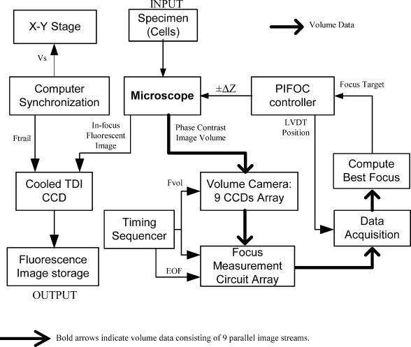 2.1.Cells and StainingNational Institutes of Health (NIH) 3T3 mouse fibroblasts (ATCC CRL 1658) were cultured at on #1.5 washed and autoclaved coverslips in and minimal essential medium with Earle’s salts, 10% fetal bovine serum, gentamicin, and L-glutamine for several days prior to fixation and staining to create an evenly distributed monolayer. They were then fixed for in 95% ethanol and air dried. The slides were stained for with a ,6-diamidino-2-phenylindole dihydrochloride (DAPI) nuclear stain solution consisting of DAPI, 10-mM Tris, 10-mM EDTA, 100-mM , and 2% 2-mercaptoethanol as described in Ref. 32. The coverslips were then laid down on cleaned microscope slides with excess DAPI solution, and sealed with nail polish. 2.2.MicroscopeThe continuous-scanning autofocus instrumentation was added to a modified Nikon Diaphot-300 inverted microscope with Plan Ph1 DL, Fluor Ph3 DL, and Plan Fluor Ph3 DLL objectives, with the 0.52-NA condenser. The objectives were designed for both phase contrast and fluorescence illumination modes, the Fluor objectives have fluorite optical elements for high UV transmission, and the Plan objectives are flat field corrected. Depth of field and NA are interrelated and are application dependent (specimen thickness). The depth of field is proportional to the wavelength, and is inversely proportional to the square of the NA.15 It is not uncommon to observe specimens thicker than the depth of field of objectives with . So submicron errors in focus can cause substantial image degradation.5 For the objective, the depth of field was , using the Rayleigh criterion in fluorescence with .15 We tested autofocus in brightfield, darkfield (not reported), and phase contrast. For the experiments reported here, autofocus was carried out using phase contrast illumination while simultaneously imaging in fluorescence by splitting the light to a different path, as shown in the light path diagram in Fig. 3 . Autofocus can be performed directly with fluorescence images, but performance is better in phase, and because of possible photobleaching and toxic fluorescence by-products, it is best to minimize fluorescence exposure, especially for live cells.8 Bright field illumination is also often brighter than fluorescence, which simplifies providing adequate signal to the nine sensors in the volume camera. For fluorescence, we used a DAPI epifluorescent filter cube (Chroma Technology, Brattleboro, Vermont) that included a excitation filter, a 400-nm dichroic mirror, and no emission filter. It was followed by a 615-nm longpass dichroic mirror (Chroma Technology, Brattleboro, Vermont) that we used to replace the 20/80 eyepiece/sideport beamsplitter prism inside the base of the microscope. This second dichroic mirror separated the phase contrast illumination from the fluorescent light; the fluorescent light was imaged at the sideport and phase contrast on the trinocular head camera port above the eyepieces. Two autofocus light sources were used: a high-luminance Hewlett Packard LED (HPWT-MH00, 626-nm wavelength) and the standard Nikon 50-W halogen bulb in conjunction with a red 665-nm cutoff longpass glass filter (Melles Griot RG665). The halogen bulb was brighter, but the LED can be strobed, and much brighter LEDs are now available. A Nikon 0.9 to C-mount zoom lens was used to couple the volume camera to the microscope’s trinocular port. 2.3.Computer Interfaces and Software ToolsThe dynamic autofocus system was controlled with a Dell Precision 220 computer with two 733-MHz CPUs, 256-MB RAM, and two 30-GB Ultra ATA/66 IDE hard drives. Two National Instruments (Austin, Texas) PCI boards were used to communicate with the external hardware: the digital IO board model PCI-DIO-96 and a data acquisition board model PCI-6031E provided connections to the focus measurement circuit array, the objective positioner, and the fluorescent-imaging CCD camera line scan timing. Focus was adjusted by a Polytec PI (Irvine, California) piezoelectric objective positioner (PIFOC) that was attached via a custom-machined adapter (that replaced the standard objective nosepiece) and driven with a Polytec PI E610 controller-amplifier. A National Instruments PCI-Step-4X motion controller board and a New England Affiliated Technologies (NEAT, Lawrence, Massachusetts) 102 microstepper driver were used to control the NEAT XYMR 60-60 motorized stage, which was fitted with a Q3DM (San Diego, California, now owned by Beckman Coulter Incorporated) slide-leveling insert. Images from the fluorescent imaging were captured with a Hamamatsu ORCA 100 TDI CCD camera and digitized by a Coreco PCI-DIG framegrabber board (Billerica, Massachusetts). The software was written in Microsoft Visual Studio 6.0 running on Microsoft NT 4 Service Pack 6. The graphical user interface (GUI) was built with Microsoft Foundation Classes (MFC). National Instruments NI-DAQ version 6.5 and Value-Motion motion version 5.0.2 libraries were used for the digital I/O, A/D, and motion control hardware. The Coreco ITEX-Core libraries (version 2.8.0) were used for fluorescence image acquisition. The Hamamatsu ORCA 100 camera (trailing camera in Fig. 3) was controlled through the software purchased with it. 2.4.Volume Camera and Focus Measurement Circuit ArrayThe volume camera captures multiple image planes at predetermined focal depths. During calibration, the focal depth for each image detector is adjusted to focus at corresponding predefined planes in specimen space, as shown diagrammatically in Figs. 1 and 3. To capture nine focal planes in parallel, the volume camera was composed of a custom array of CCD cameras fiber optically coupled to the microscope image output on the trinocular head of the microscope. The 18.8-cm-long and cross sectional area fiber optic image conduits were bundles of optical fibers custom made by Incom (Charlton, Massachusetts). (Several fiber optic companies were approached, none who had received a similar request for our long, narrow, high-quality imaging bundles, the manufacture of which was deemed challenging. More typical shapes are wide and short for conduits on the photon side of electron-photon transducers and/or tapers for changing magnification.) The light transmission efficiency of each fiber optic bundle was about 50%. Each bundle was bonded to an EG&G (Sunnyvale, California) model TD1096 ( pixels) time-delay-and-integrate (TDI) CCD sensor (capable of up to 15-MHz operation) by Photometrics (Tucson, Arizona). Each CCD sensor integrated the signal over 96 lines, thereby increasing signal-to-noise ratio [(SNR) or sensitivity] about 80-fold according to Dalsa (Waterloo, Canada) specifications. We designed and built our CCD cameras to meet the physical design constraints of placing multiple cameras in close proximity. The CCD circuit board design was simplified by use of a monolithic CCD analog signal processor chip (XRD4411 EXAR, Fremont, California), which simplified camera construction but limited pixel clock speed to or line rate. Further information on the design of these cameras is available elsewhere.33 The analog video signals from the TDI CCDs were transmitted to an array of focus measurement circuits. These focus measurement circuits enabled autofocus precision of with a objective in static autofocus in previous studies.7, 33 The data from each focus measurement circuit included: 1. the analog focus index, 2. the analog average illumination, 3. two digital gain bits (for automatic focus index gains of 1, 10, and 100), and 4. a focus-valid digital signal or trigger bit. When the focus measurement circuits operate in parallel, the amount of data supplied to the computer is composed of 18 analog signals (nine focus indices and nine average illumination values) and 27 digital bits. Once the valid focus trigger is active, the focus data remains valid for a programmed number of scan lines (typically 20 lines), enough time for a host computer to complete the acquisition operation. In addition to the CCD electronics, the volume camera system included: mechanical supports for strain relief of the fiber-CCD-sensor bonds, an integrated adapter for coupling to the microscope trinocular port, micropositioner screws for adjusting the axial position for each fiber imaging face, and electrical connectors for power and signal. Microscope optics are not perfectly flat field, so adjustable axial positioning of each imaging fiber was critical for setting actual foci during calibration. The small cross sectional area of the TDI CCD sensors does not provide for a strong bond. Mechanical strains can easily break this bond. Therefore, the fiber optic mechanical supports were mounted directly to the CCD circuit boards to uncouple the CCD-fiber bonds from mechanical forces, thereby providing a strain relief system. Low insertion force CCD sockets permitted easy removal and insertion of the board, and allowed “walking” during thermal cycling. Along with thermal gaskets, the mechanical supports also provided the heatsinks necessary for long-term operation. This design enabled a complex set of fiber optic and CCD components to function as a single volume camera with adjustments for focusing each camera fiber optic unit. 2.5.Virtual Frame and Hardware SynchronizationTo synchronize the TDI CCD sensor boards in the volume camera array, an external pulse (start of line) was sent to all cameras by a timing sequencer board, which establishes the beginning of a horizontal scan line and set the volume camera line rate ( in Fig. 2). This pulse was also transmitted to the focus measurement array, as shown in Fig. 2. Since the line scan CCDs of the volume camera produced a video signal with only horizontal blanks between video lines, the concept of end-of-frame (EOF) was absent (no vertical blank sync). Therefore, to define a focus measurement interval or virtual frame that consisted of a predefined number of lines, the timing sequencer board created and transmited an end-of-frame signal to the array of focus measuring circuits (EOF in Fig. 2). The timing sequencer worked as the central controller of the parallel focus circuits and the array of TDI cameras, synchronizing the focus measurement and acquisition of the volume camera image planes. The virtual frame shown in Fig. 4 is a subfield, or a fraction of the field of view of the specimen that moves across the CCD sensors as the stage moves. Each virtual frame first crosses each of the volume camera CCD sensors in succession and finally reaches the trailing camera. Therefore, there is a spatial offset in the focus measure of each imaging channel, which was taken into account in the control software that buffered the data and images and performed the best focus calculations. The focus measurement electronics design limited the virtual frame size to a minimum of two 1024-pixel lines, and a size of 64 lines was found to be the best tradeoff between more rapidly updating focus (less lines of integration) versus increasing SNR (more lines). Fig. 4The virtual frame corresponds to a number of 1024 pixel-wide video lines that produce a single focus measurement, and its length can be smaller or larger than the 96 lines of the TDI CCD. Image data moves across the active area of individual volume camera fibers and the trailing camera simultaneously. Focus measurements are acquired asynchronously and registered spatially for best focus comparison. The nine fibers and the trailing camera active areas are physically laid out within the full microscope field of view.  2.6.Trailing Camera and Stage SynchronizationDuring dynamic autofocusing and scanning, the resulting in-focus trailing fluorescent image was collected by a Hamamatsu (Bridgewater, New Jersey) ORCA 100 TDI cooled CCD camera with pixel size and 1280(H) 1024(V) physical pixels. In TDI mode, the horizontal resolution for this camera was firmware limited to 1024 pixels. The fluorescent imaging data stream was then broken into individual images by the ORCA camera software and framegrabber buffering system. The resulting 1.0-MB fluorescent images were stored on the hard drive for later processing and analysis. With different pixel sizes and magnifications in the relay optics, the volume and trailing cameras required different line rates to synchronize them to stage motion. These relationships are characterized by where is the stage speed, is the line frequency of the trailing camera, is the trailing camera pixel size, is the total magnification to the trailing camera port, is the line rate of the volume camera, is the volume camera pixel size, and is the total magnification to the volume camera. The software set the stage speed to conform to the rate defined by the timing sequencer hardware of the volume camera and enabled a system counter to drive TTL pulses at the appropriate line rate for the trailing camera. The velocity and magnification were adjusted and synchronized to achieve Nyquist sampling of the optical resolution at the trailing camera.2.7.Simultaneous Imaging Paths and Focus Tracking ExperimentsWith the simultaneous use of two independent imaging paths that had different electro-optical components, one for autofocus and the other for the in-focus image capture, focus and image capture calibration/synchronization was required. Even though the two microscopy modes (phase and fluorescence) share the optical path from the specimen, dividing them into two sets of sensors resulted in the need to calibrate for parfocality and centration, and synchronize acquisition in a manner that compensated for differences in sensitivity and magnification. A prescan calibration was carried out for each set of experimental conditions to obtain adequate signal levels for both output paths and compensate for positional errors caused by optical aberration and mechanical focus differences between the two light paths. Calibration was first carried out with a structured pattern as the input object (e.g., a Ronchi ruling) with its respective image observed in the output ports. When the line features were positioned parallel to the direction of stage travel, no stage motion was necessary to create a 2-D TDI image. Images were also obtained from other specimens by strobing with the LED while in TDI mode. The Hammamatsu Orca 100 CCD trailing camera was operated in full frame mode (as a static imager) for some of the alignment procedures; incremental autofocus was carried out using conventional image cytometry methods such as comparison with static autofocusing and for manually leveling the slide to within the range of the PIFOC. The detailed calibration procedures were as follows.
Fig. 5A set of calibration plots consisting of the focus measurement responses of each of the channels is shown. The normalized focus function responses of the fiber optically coupled imaging channels were obtained using a period micrometer under brightfield microscopy and a axis through focus excursion of . Channels 3 and 7 are not shown. The trailing camera focus response is also shown, and during calibration its peak is adjusted to the middle of the focus search range. 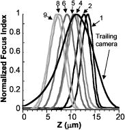 After this calibration of the imaging paths, closed-loop autofocus performance was evaluated in static- and moving-stage experiments to determine the stability of: static focus with no stage motion, dynamic focus with no stage motion with perturbations provided by manual defocus (data not shown), and tracking tilted artificial (Ronchi rulings) and cell monolayer specimens during lateral stage motion. The fluorescence image was stored for later analysis, and the volume camera signal was used only for focus tracking (in phase contrast). During scanning, a log of the objective lens positions was recorded along with the time of each recording. The time recordings enabled the percentage of focus updates missed (likely due to operating system uncertainties) to be calculated. A missing objective lens position meant a failed focus update at the unrecorded time point. The throughput of the system in cells/s depended on the cell density, the speed of the stage, and sampling density. The trailing camera recorded the continuous fluorescence image in a sequence of image frames of pixels, and this frame size and the stage speed was defined as the imaging field rate (and corresponds to a conventional 2-D or incremental imaging rate). The measurements of cell features were performed field by field on these images by a software module that can work either off-line or asynchronously with image acquisition via an on-disk image storage buffer. 2.8.Calibration of Fiber Optic Foci Before ScanningCalibrating the axial displacements (or foci) of the fiber optic imaging bundles of the volume camera was important for autofocus in continuous scanning. The axial range for calibration and operation defines the “search range” for focus measurements. Calibration of this configuration was performed using focus response curves: focus measurements of each imaging channel in the volume camera were plotted as a function of focus positions, as shown in Fig. 5. The locations of the peaks determined the axial foci of the fibers. While imaging the same flat specimen in all of the volume camera fiber channels, the relative position of each fiber face was shifted until the focus function maxima appeared at the desired axial positions to achieve the desired pattern of image sampling planes. The center fiber was routinely chosen as the reference fiber for positioning the foci of the others and calibrating the focus of the trailing camera. A staircase pattern “search range” of was typical in the specimen space. The axial magnification is approximately dependent on the square of the lateral magnification, but this dependence is asymmetrical about a given focal plane. The nonlinear magnification and the optical field curvature are probably what yielded asymmetrical and uneven real spacing between fiber faces for an evenly spaced pattern of foci in the specimen plane (see Fig. 5 for an example pattern of measured best foci). Focus measurement circuit gains were adjusted and software constants recorded to compensate for differences in response. During calibration and before starting a new scan, the slide was leveled interactively using adjustment screws on three of the corners of the slide insert in conjunction with sequential imaging of three positions (two corners and the center of the opposite side) of the rectangular scan area. This routine leveling procedure was quick and brought all of the corners within the PIFOC dynamic range. The first focus plane of the scan was set in the middle of the PIFOC range to allow for focus excursions. 3.Control System Design for Fiber Optic Continuous AutofocusThe control system software communicated with the hardware elements to close the autofocus feedback loop and acquire the fluorescence image. The control system was organized into five software modules that are designated M1 to M5 in Fig. 6 . These five modules managed the complexity of several components running in parallel, organized multiple data streams, and minimized and managed delays in the feedback loop. The nine continuous focus data streams from the volume camera were stored dynamically in multiple raw data acquisition buffers. Data were sorted via a virtual moving window (defined in software). The data was field of view (FOV) registered and placed in focus index and position buffers for best focus calculation. Software modules M1 to M5 and the data buffering relied on classes and the main National Instruments interface functions, and are described in further detail as follows. Fig. 6This data flow diagram for the real-time asynchronous software modules shows the processing of a specimen to extract a data store of images and cell biology features. The focusing feedback loop and trailing camera TDI acquisition occur simultaneously and are linked through timing signals based on stage movement velocity. Labels M1 to M5 designate the corresponding software modules.  3.1.Module M1: Volume Focus and Position Data AcquisitionModule M1 in Fig. 6 asynchronously acquires and buffers: 1. the raw volume data from the focus measurement circuit array, 2. the position from the internal LVDT sensor of the PIFOC, and 3. the focus target input to the PIFOC controller (the latter is used for diagnostics). The volume data were acquired asynchronously because the National Instruments boards did not have enough trigger inputs for acquisition to be driven independently from each of the nine channels. The National Instruments driver provided a low-level analog function class and a low-level digital function class that clocked the system and buffered multiple A/D conversions.34 For digital I/O, there is a “block transfer” subclass that groups a number of ports for handshake buffered transfer operations. For A/D input, the National Instruments software performs DMA transfers over the PCI bus directly to system memory of the PC workstation. A sequence of the analog and digital interface functions achieved the continuous acquisition. All analog functions were carried out by the PCI6031E board and all the digital functions by the PCI-DIO96 board. There are a number of setup parameters for both, but each acquisition has two main functions for the continuous data acquisition loop: a start of the data transfer and a progress of the operation check. Both the digital and analog data acquisition processes use one of the PCI-6031E analog board’s digital counters to generate TTL pulses to trigger the analog and digital data scan sequence. At each digital counter clock pulse, the digital I/O board simultaneously samples 27 digital bits (two autogain bits, and the data-valid bit from all nine autofocus circuits) or 4 port bytes, while the analog board starts a scan sequence of 20 word-sized ( each) analog channels. The A/D acquisition rate, clocked using this counter, was such that three valid focus index samples were collected from each autofocus board during every virtual frame, which was equivalent to reading each signal input ten times during a virtual frame interval. The simple strategy of three-fold oversampling of the focus valid period worked well to ensure synchronization of the low-level analog and digital data-acquisition buffers. Delays of one sample difference were observed systematically (probably due to board level hardware-driver operation); therefore, oversampling the focus signal always resulted in at least one corresponding valid analog focus value sample. The raw data acquired by National Instruments hardware were stored (through the DMA transfer) in two addressable PC memory buffers: one stored the stream of digital bits and the other the stream of analog voltages from the focus measurement circuit array. These buffers had their data elements interrelated, and a predetermined amount would correspond to one acquisition trigger; also, a software moving window was used in module M2 to search inside these data buffers. All of these values were indexed with respect to a single counter. The full length of the buffers was a function of the image sampling density, the number of video lines per virtual frame, and the length of the strip to be scanned. In a virtual frame size, we get ten samples for each signal data input, and the sizes of these buffers per focus update are There are of analog data and of digital data taken to the raw acquisition buffer for each focus update. Since the timer clock supplied a precise sample period of (focus-measure-interval/10), the data transfer rate used very little PCI bus bandwidth.3.2.Module M2: Focus Data SortingModule M2 sorts the valid focus data from invalid data in the raw focus data stream acquired by module M1. It works on one block of raw data at a time by using a moving window scheme, where the size of each block of data is the length of a virtual frame. Since the National Instruments software provides a function that checks the number of digital elements acquired, M2 begins sorting a new block of data when this function indicates that enough elements, corresponding to completion of acquisition of the most recent virtual frame, are available. As an alternative for the fast focus update, we implemented a “just in time reverse sorting” that looked for triggers immediately preceding the most recently acquired valid data point from channel 9. Because the valid triggers are roughly evenly spaced from trigger to trigger, the most recent valid data from channel 9 represents a new virtual frame that has been completed. 3.3.Module M3: Best Focus Processing and Focus UpdateSoftware module M3 aligns the focus data to compensate for the time delays caused by adjacent placement of the fiber optic bundles and registers FOVs. This module also corrects for the differences between the focus responses of the nine imaging channels of the volume camera, calculates best focus, applies a gain factor to the focus deviation to calculate a new focus target position, and provides the focus target to the PIFOC controller. The spatial arrangement of the fiber optic bundles created time delays between the nine focus data streams. Compensation for the delays was incorporated into the power-weighted average equation used in previous incremental scanning7, 8 to calculate the best focus position, where is a fiber bundle index, is the power weight, is the field of view index (for the virtual frame over which a focus measurement is made), is the spatial delay in frames from the reference fiber, is the delay-compensated focus measurement from the data stream, is the axial position of the PIFOC over the focus measurement period, is a Boolean operator for enabling or disabling a fiber channel, is the offset of fiber with respect to center fiber, and adjusts for the differences in focus response between fiber channels. Each hardware and software component has the potential to introduce delays in the feedback loop that alter the control characteristics. The position cannot be moved all the way to the new best focus at each update, because a controller that tries to eliminate errors too quickly overcorrects and becomes unstable.35 To prevent this, each new focus target position is generated bywhere is the predicted best focus from Eq. 4, is the center fiber current position, and is the feedback gain constant (which is to modulate the dynamics). Focus target positions are updated by module M3 after a new virtual frame focus data block is processed, usually several times per conventional microscope field of view until the strip is completed. The code was fine tuned to minimize the delay between reading the most recent focus measurement and repositioning focus.3.4.Modules M4 and M5: Fluorescence Image Acquisition, Image Queue, and ProcessingWhile the control system autofocuses, the high-resolution Orca 100 cooled CCD acquires the fluorescent image. The imaging line rates of the two cameras are related by Eq. 1, which matches the magnification-velocity relationship for each part of the experimental setup, including different objectives. In the experiments reported here, the fluorescence image queue was stored on the hard drive and processed at a later time. However, image segmentation, processing, feature extraction, and analysis were previously implemented,36, 37, 38 have been commercialized in the Q3DM-Beckman Coulter IC-100 CytoShop software, and could operate directly on the buffered images as they are acquired, as shown in Fig. 6 (by the dotted arrows), to complete processing analyses and feature extraction more rapidly. After segmentation of the cell nuclei, border cell artifacts (cut fragments of nuclei) were removed and the integrated intensity (DNA content) of each nucleus was stored. 3.5.Continuous-Scanning SequenceThe continuous-scanning sequence is initiated by accelerating the stage to the predetermined scan velocity before starting the volume and TDI trailing camera image acquisition, as depicted in Fig. 6. For each block of focus data, a process loop sorts the raw data, calculates best focus, and repeatedly moves the objective until the entire strip is acquired, achieving the autofocus loop. The TDI trailing and volume camera acquisitions are halted, the stage is retraced, and parameters are set for the next strip. This sequence is repeated to acquire as many strips as needed to scan the predetermined area. The system response was studied by measuring the average software process execution times from repeated scans (Table 2 ). Table 2Software execution and latency timing. “a” denote strip size (mm)/stage speed (mm/s). * depends on moving window size. “b” depends on objective positioner calibration. “c” dependant on system hardware latencies. NM is not measured. “d” much less than the time to position stage and objective to new positions. Processes 4 through 7 represent the autofocus loop.
4.ResultsFirst, an analysis of the software and hardware latencies was carried out, since these are fundamental to the feedback characteristics of the system. These latencies include the time required for software sorting and processing, the PIFOC response, and the time delays caused by the sequentially lateral displacement of the fiber optic imaging faces. The complexity of the parallel hardware system latencies was managed by synchronization in the software modules to enable closed-loop autofocus. Table 2 lists the software modules along with their indexed processes, execution times, order of execution dependency, and state interdependencies. The timing-critical software functions were: sorting the data, calculating best focus, and checking progress of the moving focus-image acquisition window. The sorting function proved to be the slowest of the processes, but was still 2 orders of magnitude faster than closed loop electromechanical objective repositioning (PIFOC response of ). Calculating the best focus and checking the scan progress, which were performed for each feedback adjustment of the objective focus position, required 10% the overhead of the sorting function. The system design thus successfully limited and managed these latencies, and understanding them helped in setting the feedback gain. Static- and moving-stage experiments were carried out to better understand the effects of the latencies, determine the best gain settings, and characterize the closed-loop autofocus performance. In the static-stage experiment, the microscope stage was immobile, but environmental conditions including mechanical vibrations and thermal focus drift were present. Closed-loop autofocus was performed at a focus update rate of , and the static-stage focus position was maintained with a SD of over a 70-s period. In the moving-stage autofocus experiment, a comparison of tracking on a moving, tilted slide with etched Ronchi rulings (of ) in continuous and incremental autofocus is shown in Fig. 7 . Focus was updated up to every along the direction of stage travel with the objective. Increasing the focus update gain in Eq. 5 improved tracking later in the scan, but higher gains demonstrated more oscillatory behavior at the beginning. There can be transient out-of-focus instability or drift at the beginning of the scan because the focus measurements are in error until the stage reaches a constant velocity and traverses the distance between the outer fibers. This was corrected by a prestart period of acceleration where autofocus is not performed. Fig. 7Continuous focus tracking over of a tilted specimen at different gains is compared to incremental focus (at four positions). Ronchi rulings of were imaged with a Fluor 160-mm tube length objective at a stage speed of . Focus was updated at with a focus update distance of .  The ultimate goal was to acquire in-focus fluorescent images of cells during continuous stage motion using on-the-fly focus tracking. Continuous fluorescence imaging was broken into image frames of pixels , and an image strip was composed by the concatenation of these frames. This is demonstrated with the fluorescence image shown in Fig. 8a , which is a typical sharp image strip acquired during continuous scanning of DAPI-stained cells cultured on a coverslip. Focus tracking of cells on four 30-mm-long strips included more than 5700 focus updates, of which only 1.74% were missed for an average of one miss every 57 fluorescence images. The scanned area comprised more than 700 1-MB fluorescence images. Focus was measured and updated just over 8 times per one fluorescence image field captured with the trailing camera, or 8-fold more often than with our incremental scanning system. For this reason, the occasional failure to update focus was not thought to compromise autofocus performance. As can be seen in Fig. 8b, focus tracking was well behaved and study of the data revealed no unexpected behaviors associated with missed update misses. The speed of the stage in these experiments was or with fluorescence image sampling of , which resulted in a field rate of . In other similar cell scanning experiments, the stage speed was set to and a fluorescence image sampling of , providing an imaging rate of . We achieved a maximum focus update rate of reliably; failure to update focus started to increase beyond this value. The stage speed was limited to by the prototype volume camera line rate, which corresponded to a fluorescence field rate of with the objective. All of the captured images were sharp, indicating that dynamic autofocus performed well. Fig. 8(a) A fluorescence image strip acquired with a resolution of is shown. The left strip represents a 4-mm length of the specimen. The right image is a area and 24 focus updates occurred on it as shown by the marks along the right side of the image. These images were extracted from a 30-mm-long continuous scan of NIH 3T3 cells cultured on a coverslip and stained with DAPI. Stage speed was (for ). With an ideal, densely populated specimen , these conditions would scan up to . (b) A plot of the focus positions over the full 30-mm scan is shown. The focus update rate was . The images were acquired with a Plan Fluor Ph3 objective. The stage speed was and it took to scan the .  Table 3Summary of performance of the new continuous scan and autofocus system. “a” Test conditions: closed-loop autofocus with no stage motion. Specimen: Ronchi rulings (2000lines∕in.) , focus update rate= 27Hz . Microscope in brightfield mode, tests were carried out with 20× and 40× optics, and focus feedback gain of 0.2 and 0.4. “b” Specimen: NIH 3T3 cells with DAPI stain. There were 769 cells detected, mostly in the G0 phase.
Table 3 summarizes the experimental conditions and performance results for continuous scanning and autofocus. The autofocus error was obtained from several 70-s-long closed-loop autofocus trials, which were carried out at an update rate of with the stage not moving. For all of the trials, the error was the standard deviation of the focus position, and the “best” experiment was the one with the lowest standard deviation. For the G0/G1 CV reported in Table 3, commercial DNA analysis software (Phoenix Flow System, San Diego, California) was used to fit the DNA content histogram measurements that were performed on a section of a slide on which NIH 3T3 cells were cultured and stained with DAPI. 769 cells were detected and focus tracking performed well (with a stage speed of ), even with the relatively low cell density. 5.Discussion and ConclusionsThis combination of optics, electronics, and software control functions successfully achieved closed-loop continuous-image-content-based autofocus on a microscope for the first time. Careful design, testing, and calibration were critical for determining the delays and divergence of focus responses in each channel and compensating in software for these differences. The software control system provided functions for calibration, buffering, and processing the raw data, measuring and maintaining closed-loop feedback autofocus, and acquiring the fluorescence image. Sharp focus of cell monolayers on microscope slides demonstrated that parallel multiplanar focus measurements are a powerful basis for autofocus in TDI image acquisition for microscopy. The high static focus precision of resulted from simultaneous focus sampling of multiple focal planes, enabling a much higher effective focus measurement rate. This precision was consistently better than the best SD of and the average of that we previously achieved in sequential autofocus.7 The absolute focus positions of dynamic autofocus matched the incremental autofocus carried out on the same field of view well. In comparing dynamic autofocus positions to those obtained during incremental scanning, repositioning errors due to system thermal and mechanical instabilities are likely on the order of , so caution must be used in overinterpreting the results in Fig. 7. Given the repositioning errors, the different gains tracked the specimen well and it can be concluded that decreasing the gain enough to eliminate oscillation resulted in good tracking for specimen gradients within (for the experiments of Fig. 7). Furthermore, for a typical focus search range (or vertical sampling of the fiber optic staircase in specimen space) of , continuously tracking a specimen slope of worked for all of the slides we prepared. The system was tested with , , and objectives. Autofocus is simpler with lower NA objectives where depth of field is larger. Performance was also excellent on the higher 0.75-NA objectives, confirming that this image-content-based autofocus system is also capable of performing well with higher resolution objectives. Autofocus performance better than the depth of field for a range of objectives will enable a broad range of applications. The seven software modules operated concurrently under Windows NT. The raw tracking data were collected asynchronously in the background using the National Instruments boards and DMA transfers, which do not require CPU overhead. The tracking data acquisition memory requirements were manageable, and the computer was fast enough to carry out the software processes without requiring explicit real-time operating system functions. Even though acquiring the tracking data asynchronously from the focus measurement circuit data-valid signal is inefficient because both valid and invalid autofocus data are acquired and a search is required to locate the valid data, this extra overhead was not limiting. This practical buffering and sorting solution prevented the additional headaches of software design for specialized real-time operating systems and synchronous hardware interfaces. The penalty was an average of one missed focus update for every 57 conventional 2-D fields of view, which did not appear to adversely affect autofocus performance. Another possible reason for these occasional missed focus updates was the moving window jitter, which was previously noted to omit the reading of buffered samples during the valid focus trigger. However, short term measurements indicated that only one of the three valid buffered samples was missed due to window jitter, which would not have prevented the system from updating a new best focus. But it is possible that all three samples were missed very rarely. Whatever the source of missed focus updates, focus was updated frequently enough (8 times/conventional 2-D field) to keep the high-resolution fluorescence image sharply focused during continuous stage motion. The lateral offsets between fields of view (or virtual frames) of the fiber optic imaging faces in the volume camera required buffering and registration for correct comparison of focus measurements and continuous focus tracking operation. These offsets introduced a delay that slowed tracking response and might adversely affect performance under conditions not yet demonstrated. The delay may reduce tracking response to sharp transient gradients in the specimen surface. Direct use of the measurements without registration increased the response to sharp gradients, but also increased uncertainty around best focus position (data not shown). It is possible that a feedback model that explicitly accounts for these different delays might perform better than the proportional feedback model implemented here. A related problem is that a linear staircase pattern for the axial positions of the fiber faces might coincidently be exactly matched by a long linear specimen gradient. At the appropriate velocity, this condition would yield no focus measurement differences at best focus on which to base feedback control, which might in turn lead to oscillatory behavior not yet encountered. A staggered pattern of the fiber faces would reduce the probability of encountering a specimen-fiber optic gradient match. Other possible disadvantages of the imaging fiber bundles were: their fragility (especially the small-area glued CCD-bundle interface), errors in magnification due to variation in the packing density, degradation of the imaging MTF, irregular CCD-to-fiber bonding distance, end-to-end cross sectional area mismatches, loss in image transmission, and occasional defects that introduced fixed distortion patterns. Overall, however, the fiber imaging quality was high and these defects, which probably largely produced variability in the noise floor between imaging channels, did not appear to greatly degrade performance. It is instructive to estimate possible cell analysis rates using the principle of continuous TDI scanning. Cell density varies and increased cell density can add complexity to image segmentation,39 but with a densely populated specimen of, e.g., white cells smeared on a slide at (allowing ), the present experimental conditions would result in a rate of about . And at the maximum line rate of permitted by the volume camera prototype (or for the trailing camera) and a objective (versus the objective in these experiments), the rate would be . Further increases in line rate or CCD line length would proportionally increase analysis speeds. The 4-kHz maximum line rate of the volume camera should result in a maximum focus position update rate of lines/focus , which is still below the characteristic PIFOC controller system frequency of about (or a 10-ms response period). In our experiments, we achieved a maximum update rate of reliably. Successful closed-loop feedback autofocus in continuous-motion scanning enabled high-resolution image cytometry operation at speeds more comparable to flow cytometry. Sequential start-and-stop stage motion and focus measurement in conventional automatic image cytometry previously placed substantial limitations on both speed and imaging efficiency. Imaging multiple focal planes in parallel and acquiring the fluorescence image at the same time enabled continuous scanning that overcame the image cytometry limitations (microscope stage acceleration and sequential imaging of the focal planes for autofocus) of incremental scanning. With continuous scanning, image acquisition speed is limited only by the combinations of camera sensitivity, fluorescence intensity, and CCD line width. For bright fluorescence, scanning speed will continue to increase with faster CCD clocking. And for any given fluorescence brightness and optical setup, increasing the CCD line width will result in a directly proportional increase in speed through adding imaging parallelism, limited only by the objective field of view. Using the most recent Nikon infinity-corrected objectives, Nyquist sampling with 1,024-pixel video lines acquires an image comprising about 1/3 of the field of view. Longer CCD lines will proportionally increase scanning speed at the same brightness. Thus, increasing parallelism is a powerful tool that can continue to be exploited for further increases in scanning speed. Many cells can be imaged and analyzed in parallel with continuous-motion image cytometry, whereas flow cytometry has been limited to sequential operation or a single file stream of cells thus far. If this fundamental difference persists, image cytometry speed can continue to increase as technologies improve without sacrificing sensitivity, while flow cytometry speed increases will be fundamentally limited by single-file sequential cell measurement operation. With both the speed and information advantage, we predict that image cytometry instrumentation will eventually supplant flow cytometry, especially for applications where the cells are natively anchorage-dependent. AcknowledgmentsThe authors would like to thank Benedikt v. Massenbach, Francis Nguyen, Jose Sanchez, and Sam Bae of University of California, San Diego, for their help with the system implementation, and Lisa O’Brien for assistance with manuscript preparation. This research was supported by a Whitaker Foundation Biomedical Engineering Research Grant, the University of California Institute for Mexico and the United States (UC-MEXUS), the Consejo Nacional de Ciencia y Tecnología de México (CONACYT), National Science Foundation Major Research Instrumentation grant BES-9871365, and NIH NIBIB grant 1 R01 EB006200. M. Bravo-Zanoguera thanks the CONACYT for the scholarship support. ReferencesH. Shapiro, Practical Flow Cytometry, 3rd ed.Wiley-Liss, New York (1995). Google Scholar
S. Bajaj,
J. B. Welsh,
R. C. Leif, and
J. H. Price,
“Ultra-rare-event detection performance of a custom scanning cytometer on a model preparation of fetal nRBCs,”
Cytometry, 39
(4), 285
–294
(2000). https://doi.org/10.1002/(SICI)1097-0320(20000401)39:4<285::AID-CYTO6>3.0.CO;2-2 0196-4763 Google Scholar
M. R. Koller,
E. G. Hanania,
J. Stevens,
T. M. Eisfeld,
G. C. Sasaki,
A. Fieck, and
B. O. Palsson,
“High-throughput laser-mediated in situ cell purification with high purity and yield,”
Cytometry, 61
(2), 153
–161
(2004). 0196-4763 Google Scholar
M. Bravo-Zanoguera and
J. H. Price,
“Simultaneous multiplanar image acquisition in light microscopy,”
Proc. SPIE, 3260 184
–200
(1998). 0277-786X Google Scholar
M. Bravo-Zanoguera,
B. von Massenbach, and
J. H. Price,
“Automatic on-the-fly focusing for continuous image acquisition in high-resolution microscopy,”
Proc. SPIE, 3604 243
–252
(1999). https://doi.org/10.1117/12.349206 0277-786X Google Scholar
M. Bravo-Zanoguera,
B. von Massenbach,
A. L. Kellner, and
J. H. Price,
“High-performance autofocus circuit for biological microscopy,”
Rev. Sci. Instrum., 69
(11), 3966
–3977
(1998). https://doi.org/10.1063/1.1149207 0034-6748 Google Scholar
J. H. Price and
D. A. Gough,
“Comparison of phase-contrast and fluorescence digital autofocus for scanning microscopy,”
Cytometry, 16
(4), 283
–297
(1994). 0196-4763 Google Scholar
T. D. Harris,
R. L. Hansen,
W. Karsh,
N. A. Nicklaus, and
J. K. Trautman,
“Method and apparatus for screening chemical compounds,”
(2002). Google Scholar
Y. Liron,
Y. Paran,
N. G. Zatorsky,
B. Geiger, and
Z. Kam,
“Laser autofocusing system for high-resolution cell biological imaging,”
J. Microsc., 221
(2), 145
–151
(2006). 0022-2720 Google Scholar
B. S. Manian,
D. M. Heffelfinger, and
E. M. Goldberg,
“Optical autofocus for use with microtiter plates,”
(2002). Google Scholar
F. C. Groen,
I. T. Young, and
G. Ligthart,
“A comparison of different focus functions for use in autofocus algorithms,”
Cytometry, 6
(2), 81
–91
(1985). https://doi.org/10.1002/cyto.990060202 0196-4763 Google Scholar
L. Firestone,
K. Cook,
K. Culp,
N. Talsania, and
K. Preston,
“Comparison of autofocus methods for automated microscopy,”
Cytometry, 12
(3), 195
–206
(1991). https://doi.org/10.1002/cyto.990120302 0196-4763 Google Scholar
M. A. Oliva,
M. Bravo-Zanoguera, and
J. H. Price,
“Filtering out contrast reversals for microscopy autofocus,”
Appl. Opt., 38
(4), 638
–646
(1999). 0003-6935 Google Scholar
S. Inoué and
K. R. Spring, Video Microscopy: The Fundamentals, 2nd ed.Plenum Press, New York (1997). Google Scholar
H. Netten,
L. J. van Vliet,
F. R. Boddeke,
P. de Jong, and
I. T. Young,
“A fast scanner for fluorescence microscopy using a 2-D CCD and time delayed integration (image cytometry),”
Bioimaging, 2
(4), 184
–192
(1994). https://doi.org/10.1002/1361-6374(199412)2:4<184::AID-BIO3>3.0.CO;2-M 0966-9051 Google Scholar
K. R. Castleman,
“The PSI automatic metaphase finder,”
J. Radiat. Res. (Tokyo), 33
(1), 124
–128
(1992). 0449-3060 Google Scholar
G. Shippey,
R. Bayley,
S. Farrow,
R. Lutz, and
D. Rutovitz,
“A fast interval processor (FIP) for cervical prescreening,”
Anal Quant Cytol., 3
(1), 9
–16
(1981). 0190-0471 Google Scholar
J. H. Tucker,
O. A. Husain,
K. Watts,
S. Farrow,
R. Bayley, and
M. H. Stark,
“Automated densitometry of cell populations in a continuous-motion imaging cell scanner,”
Appl. Opt., 26
(16), 3315
–3324
(1987). 0003-6935 Google Scholar
J. H. Tucker and
G. Shippey,
“Basic performance tests on the CERVIFIP linear array prescreener,”
Anal Quant Cytol., 5
(2), 129
–137
(1983). 0190-0471 Google Scholar
J. Laitinen and
I. Moring,
“Method for evaluation of imaging in automated visual web inspection,”
Opt. Eng., 36
(8), 2184
–2196
(1997). 0091-3286 Google Scholar
S. H. Ong,
D. Horne,
C. K. Yeung,
P. Nickolls, and
T. Cole,
“Development of an imaging flow cytometer,”
Anal Quant Cytol. Histol., 9
(5), 375
–382
(1987). 0884-6812 Google Scholar
S. H. Ong and
P. M. Nickolls,
“Analysis of MTF degradation in the imaging of cells in a flow system,”
Int. J. Imaging Syst. Technol., 5 243
–250
(1994). 0899-9457 Google Scholar
T. C. George,
D. A. Basiji,
B. E. Hall,
D. H. Lynch,
W. E. Ortyn,
D. J. Perry,
M. J. Seo,
C. A. Zimmerman, and
P. J. Morrissey,
“Distinguishing modes of cell death using the ImageStream multispectral imaging flow cytometer,”
Cytometry, 59A 237
–245
(2004). 0196-4763 Google Scholar
, “Time delay integration: enabling high sensitivity detection for imaging-in-flow on the ImageStream® 100 cell analysis system,”
Google Scholar
W. E. Ortyn and
D. A. Basiji,
“Imaging and analyzing parameters of small moving objects such as cells,”
(2003). Google Scholar
D. A. Basiji and
W. E. Ortyn,
“Alternative detector configuration and mode of operation of a time delay integration particle analyzer,”
(2005). Google Scholar
W. E. Ortyn,
M. J. Seo,
D. A. Basiji,
K. L. Frost, and
D. J. Perry,
“Autofocus for a flow imaging system,”
(2005). Google Scholar
L. K. Nguyen,
M. Bravo-Zanoguera,
A. L. Kellner, and
J. H. Price,
“Magnification corrected optical image splitting for simultaneous multiplanar acquisition,”
Proc. SPIE, 3921 31
–40
(2000). 0277-786X Google Scholar
J. H. Price,
“Autofocus system for scanning microscopy having a volume image formation,”
(August 3, 1999). Google Scholar
M. Bravo-Zanoguera and
J. H. Price,
“Analog circuit for an autofocus microscope system,”
(1999). Google Scholar
S. Hamada and
S. Fujita,
“DAPI staining improved for quantitative cytofluorometry,”
Histochemistry, 79
(2), 219
–226
(1983). 0301-5564 Google Scholar
M. E. Bravo-Zanoguera,
“Autofocus for high speed scanning in image cytometry,”
(2001) Google Scholar
,
(1999) Google Scholar
V. J. VanDoren,
“Controllers balance performance with closed-loop stability,”
Control Eng., 47
(5), 104
(2000). 0010-8049 Google Scholar
J. H. Price,
E. A. Hunter, and
D. A. Gough,
“Accuracy of least squares designed spatial FIR filters for segmentation of images of fluorescence stained cell nuclei,”
Cytometry, 25
(4), 303
–316
(1996). 0196-4763 Google Scholar
J. H. Price and
D. A. Gough,
“Method and means of least squares designed filters for image segmentation in scanning cytometry,”
(Aug. 4, 1998) Google Scholar
S. Heynen and
J. H. Price,
“Evaluation of scanning cytometer fluorometry performance,”
Proc. SPIE, 3604 237
–242
(1999). https://doi.org/10.1117/12.349205 0277-786X Google Scholar
N. L. Prigozhina,
L. Zhong,
E. A. Hunter,
I. Mikic,
S. Callaway,
D. R. Roop,
M. A. Mancini,
D. A. Zacharias,
J. H. Price, and
P. M. McDonough,
“Automated image cytometry of plasma membrane proteins and DNA content for high throughput screening,”
Assay Drug Develop. Technol., 5
(1), 29
–48
(2007). Google Scholar
|


