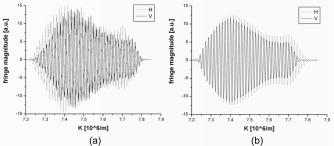
1.

Introduction

Optical coherence tomography (OCT) is an imaging technique that measures the interference between a reference beam of light and a beam reflected back from a sample.¹ Recent advancements have led to the development of spectral/Fourier-domain optical coherence tomography (SD-OCT),^{2, 3, 4} providing superior sensitivity and speed.^{5, 6, 7, 8} Ultra-high speed and ultra-high resolution have been demonstrated for in vivo ophthalmic applications.^{9, 10, 11, 12} In SD-OCT, the structural information, i.e., the depth profile (A-line), is obtained by Fourier transforming the optical spectrum of the interference as measured by a spectrometer at the output of a Michelson interferometer.^{2, 3} In swept-source optical frequency domain imaging (OFDI) systems,¹³ a point detector is used to record the intensity of the interference corresponding to individual wavelengths rapidly scanned by the swept-source, and this information is converted to a depth profile by Fourier transform as in SD-OCT. Fourier transformation relates the physical distance $\left(z\right)$ with the wave number $(k=2\pi ∕\lambda )$ . The spectra obtained with SD-OCT and OFDI are not necessarily evenly spaced in $k$ -space. A proper depth profile can be obtained only after preprocessing to obtain data that is evenly spaced in $k$ -space,³ and this requires accurate assessment of the wavelength corresponding to each spectral element for both techniques.

Determination of this wavelength mapping is typically performed using separate measurements of a reflective surface at different positions in the sample arm.^{3, 14} The importance of proper wavelength assignment for SD-OCT was first noted by Wojtkowski ³ Incorrect wavelength mapping generates a depth-dependent broadening of the coherence peak similar in appearance to dispersion in structural OCT images. The accuracy of this wavelength assignment can be even more critical for a polarization-sensitive spectral-domain OCT (PS-SDOCT) system. Qualitative PS-SDOCT has been demonstrated for measurement of skin¹⁵ and human retina birefringence.¹⁶ Quantitative PS-SDOCT¹⁷ requires a more precise calibration and removal of polarization artifacts. Cense¹⁸ already demonstrated that incorrect wavelength assignment creates artifactual birefringence. In PS-SDOCT, the interference pattern is typically split and detected in two orthogonal polarization channels.^{14, 17} Even a slight mismatch of the wavelength mapping between the two analysis channels leads to depth profiles with enough of a difference in depth $\left(z\right)$ range to create an artificial birefringence.¹⁴ A previous paper¹⁴ described a high-speed spectrometer that can be used in a PS-SDOCT system, as well as a calibration method for the spectrometer. In fact, some form of separate calibration has been necessary in all SD-OCT and OFDI systems to date. The disadvantage of such calibration methods is that they typically require separate measurements of a reflective surface. Using the example of a clinical ophthalmic system, calibration data from a model eye are acquired before or after imaging of the patient in order to later determine the appropriate wavelength mapping. The calibration procedure may be necessary for each measurement session due to thermal and mechanical instabilities of the spectrometer, which is not practical in a clinical setting. This paper describes an autocalibration technique wherein the calibration data does not have to be acquired separately but is contained within the data of interest.

2.

Principle of the Method

Proper wavelength assignment can be achieved by imposing onto the spectrum a known modulation that can be used for calibration. In the system presented here, we introduce a perfect sinusoidal modulation as a function of $k$ by passing the light through a microscope coverslip in the interferometer’s source arm. This slide creates spectral modulation by combining the light that passes directly through the glass with the light that is internally reflected twice before transmission. The interference can be characterized by an optical path mismatch of $2dn$ , where $n$ is the refractive index and $d$ is the thickness of the glass coverslip, and is in the form cos $\left(2dnk\right)$ . This spectral modulation is a perfect cosine as a function of $k$ , assuming that $n$ is independent of the wavelength for the bandwidth of the light source.

The presence of this spectral modulation is key in assigning the correct wavelength to each pixel of the CCD in the spectrometer case. In general, the pixels do not correspond to evenly distributed $k$ , and therefore, the detected intensity modulation is not a perfect sinusoid. The autocalibration technique alters the wavelength assignments until the resulting spectral modulation matches a perfect sinusoid as a function of $k$ . This sinusoidal intensity modulation produces in all A-lines an identical strong peak along $z$ corresponding to the optical thickness of the slide. This peak can be easily removed as fixed pattern noise from the structural intensity images in a patient scan.

Figure 1a shows a typical intensity modulation generated by the slide for the spectrum of a Ti:Sapphire laser (Integral OCT, Femtolasers, Vienna, Austria) with a spectral bandwidth of $150\mathrm{nm}$ centered at $800\mathrm{nm}$ . This spectrum has been obtained as the mean of 1000 spectra corresponding to one frame in a three-dimensional (3-D) patient scan. The interference fringes resulting from the structure of the scan are mostly washed out in this mean, while the fringes from the slide are unaffected. The spectral interference fringes from the slide are isolated with a bandpass filter in Fourier space, and the result is shown in Fig. 1b in the CCD pixel space. By keeping only the peak from the slide, we also remove the DC component of the spectral interference, illustrated in Fig. 1b as a zero-mean interferogram. When represented as a function of $k$ , the fringes in Fig. 1b should be perfectly periodic. For a perfect sinusoid, the phase, or the argument of the sinusoidal oscillation, is linearly related to $k$ . This condition is used to determine the accuracy of the wavelength assignment; an improper wavelength assignment results in phase non-linearity as a function of $k$ . The wavelength mapping is determined by minimizing the nonlinearity of this phase. An initial estimate of the wavelength array $W$ is generated (using the grating equation based on the geometrical design of the spectrometer,¹⁴ or alternatively, with a third-order polynomial bringing the generated wavelengths in the spectral range of the light source). $W$ is used to interpolate the spectral interference fringes to equally spaced $k$ values. The quality of this interpolation process is improved by zero-padding the spectrum.

Fig. 1

(a) Spectrum (in arbitrary units) of interference generated by the slide as a function of the index of the CCD pixels. (b) Spectral interference fringes (in arbitrary units) corresponding to the slide, shown in CCD pixel space.

The next step is to iteratively determine and apply corrections to the wavelength assignment by reducing the phase nonlinearity. The phase of the zero-padded and $k$ -space interpolated spectrum is determined and fit with a third-order polynomial. The nonlinear part $\sigma \left(K\right)$ of the polynomial fit (which has only the quadratic and the cubic dependence on $K$ and represents the deviation from a perfectly linear phase) is used for correcting the wavelengths $W$ based on the assumption that this nonlinearity is generated by wrong wavelength assignment. Therefore, we calculate a new $k$ -array $K^{\prime }$ , starting from the previous $K=2\pi ∕W$ array and $\sigma \left(K\right)$ , using the equation $K^{\prime }=K+\sigma \left(K\right)∕z\left(\text{peak}\right)$ , where $z\left(\text{peak}\right)$ is given by $z\left(\text{peak}\right)=2\pi \text{Peak}̱\text{index}∕(K_{\max }-K_{\min })$ . Peaḵindex is the location of the coherence peak corresponding to the slide in index space, and $K_{\max }$ and $K_{\min }$ are the extremes of $K$ . This correction is applied iteratively to the original spectral interference, and the final result is the wavelength array $W^{\prime }=2\pi ∕K^{\prime }$ that corresponds basically to linear phase as a function of $K^{\prime }$ . The condition to be met in order to exit the loop could be either a maximum number of iterations or a tolerance in the change of the wavelength array after each iteration. The wavelength array $W^{\prime }$ is saved for later use when analyzing the patient OCT data.

3.

Calibration of a Polarization-Sensitive Spectrometer

The accuracy of wavelength assignment can become even more important for functional extensions of OCT such as PS-OCT.¹⁴ In a polarization-sensitive spectrometer, the spectral interference is analyzed simultaneously in two orthogonal polarization channels, H and V. The procedure outlined earlier can be applied to each of the two polarization channels; however, additional steps are required to remove polarization artifacts and to ensure that the two polarization channels cover the same depth range $z$ . In principle, one intensity modulation provides enough information to yield spectra that are perfectly evenly spaced in $k$ -space. However, there is no guarantee that the fringe patterns have exactly the same $k$ -spacing in the two polarization channels or that they perfectly overlap. Introduction of a second modulation provides the additional information necessary to transform the two polarization channels’ spectra for a perfect overlap of the fringe patterns. In the polarization-sensitive case, we use two microscope slides with different thicknesses that create two coherence peaks at different positions along the depth profile in both polarization channels. In general, the peaks for the two polarizations do not overlap, as shown in Fig. 2 , at the two depths corresponding to the two slides given the mapping as obtained earlier. We keep $K_H$ and the spectrum H unmodified, and we correct for this by modifying $K_V$ , the $k$ -array associated to the V spectrum.

Fig. 2

Depth profiles for the two polarization channels showing that the peaks do not overlap: dotted line—H polarization; solid line—V polarization.

The depth position of the coherence peak is given by the frequency of the fringes in $k$ -space, which is related to the slope of the phase. All these quantities have to be the same for the two polarization channels. Therefore, the V spectrum must be modified such that the fringes have the same frequency. Since we already have the mapping for H and V, we calculate the depth $z$ for each pixel in the depth profile for both H and V ( $z_H$ and $z_V$ ). We then compare $z_H$ and $z_V$ at the two peaks and determine the percentage needed to expand or contract $K_V$ such that the coherence peaks for the two polarizations overlap at the two depths $(\text{percentage}=z_H\left(\text{peak}2\right)∕z_V\left(\text{peak}2\right))$ . A new $K_V$ is calculated, $K_V^{\prime }$ , based on this percentage ( $K_V^{\prime }=K_0+1∕{\mathit{\text{percentage}}}^{*}(K_V-K_0)$ where $K_0$ is the central $k$ value), and the V spectrum is interpolated from $K_V^{\prime }$ to $K_H$ to bring both spectra in the same $k$ -range. The result, illustrated in Fig. 3 , shows 20 times zero-padded coherence peaks corresponding to the two slides [(a) and (b), respectively] for the two polarization (dotted line—H polarization; solid line—V polarization).

Fig. 3

20 times zero-padded coherence peaks corresponding to the two slides (a) and (b) for the two polarization channels showing perfect overlap after modifying $K_V$ and the spectrum V: dotted line—H polarization; solid line—V polarization.

Even if the fringes have the same frequency, providing perfect overlap of the depth profiles, the fringe patterns should also overlap perfectly when represented in $k$ -space since the intensity modulation is the same for the two polarizations. A remaining nonzero phase difference between the two polarizations’ spectra indicates that the spectra are shifted with respect to each other, as illustrated in Fig. 4a . This incorrect wavelength assignment generates polarization artifacts, a ghost birefringence that acts as an offset in the calculated tissue birefringence, and needs to be corrected. In order to overlap the fringe patterns corresponding to the two polarizations and for the two slides simultaneously, we separate the fringe patterns for the two slides, and for each slide, we cross-correlate the two polarizations. The two cross-correlations are multiplied to determine the best simultaneous overlap and to select the pixel shift corresponding to the maximum of the product. This pixel shift is converted into a $K$ -shift that translates $K_V$ ( $K\text{-}\text{shift}=\text{pixel}{\text{shift}}^{*}k$ -spacing, where $k\text{-}\text{spacing}=(K_{\max }-K_{\min })$ /total number of $k$ -values). The two cross-correlations can be zero-padded for a more precise calculation of the $K$ -shift. The V spectrum is interpolated to the shifted $K_V$ range, and the result is shown in Fig. 4b, demonstrating perfect overlap of the fringes corresponding to the first slide. The wavelength assignments calculated from the shifted $K_V$ and from $K_H$ (that was not modified) are saved to be used when analyzing the OCT data.

Fig. 4

(a) Spectra in $k$ -space shifted with respect to each other. (b) Overlapped fringes from slide 1 for the two polarizations after shifting $K_V$ and interpolating spectrum V to the shifted $K_V$ : dotted line—H polarization; solid line—V polarization.

4.

Experimental Results

We tested this method using a series of measurements from a sample constructed of a mirror in a model eye while stepping the reference mirror by $100\mu \mathrm{m}$ in air. A schematic of the PS-SDOCT system is shown in Fig. 5 . The light source for these measurements was a superluminescent diode (Superlum, Moscow, Russia) with a center wavelength of $840\mathrm{nm}$ and a full width at half maximum (FWHM) of $50\mathrm{nm}$ . The details of the polarization-sensitive spectrometer were described elsewhere.¹⁹ In short, a Wollaston prism is used to separate the two orthogonal polarization components of the interference spectrum dispersed by a transmission diffraction grating. The resulting spectra are simultaneously imaged on the same linear CCD, each of them on a half of the CCD. This particular spectrometer design limits the bandwidth of the light source that can be used such that two spectra (for the two orthogonal polarizations) can be imaged on the linear CCD without overlap. However, our calibration method is general for any light source, and a redesigned spectrometer could also be used with a Ti:Sapphire laser for better axial resolution. The spectrometer calibration is performed as outlined earlier and provides perfect overlap of the coherence peaks for the two polarization channels, as shown in Fig. 6 , where red and blue correspond to the two polarization channels, H and V. In MATLAB, the calibration of the PS-SDOCT spectrometer takes about $10\mathrm{s}$ , and can be implemented in real time. It needs to be done just once per measurement session, and it does not require a sample (patient).

Fig. 5

Measurement setup for PS-SDOCT. HP-SLD—broadband source; I—isolator; M—polarization modulator; SL—slit lamp based retinal scanner; RSOD—rapid scanning optical delay line; PBS—polarizing beamsplitter; ND—variable neutral density filter; C—collimator $(\mathrm{f}=100\mathrm{mm})$ ; TG—transmission grating $(1200\text{lines}∕\mathrm{mm})$ ; L—photographic multielement lens $(\mathrm{f}=105\mathrm{mm})$ ; CCD—line scan CCD camera; W—calcite Wollaston beamsplitter; PC—polarization controllers.

Fig. 6

The depth decay measured with a mirror in a model eye in the sample arm. (The reference mirror was moved in steps of $100\mu \mathrm{m}$ in air.) Red and blue correspond to the two polarization channels, H and V.

The Stokes vector is calculated for each position of the mirror in the reference arm following known procedures for depth-resolved polarization analysis.^{20, 21} Figure 7 shows the angle on the Poincaré sphere between the Stokes vector at the first mirror position and all the subsequent ones. The small angular deviation demonstrates a very efficient removal of depth-dependent ghost birefringence. One can determine the error in the $k$ assignment as $\Delta k=\Delta \Phi ∕z$ based on the phase error $\Delta \Phi$ given by the Stokes vector angle error on the Poincaré sphere for a depth $z$ . The wavelength assignment error is then $\Delta \lambda ={\lambda }^2\Delta k∕2\pi$ . The average phase error for the 16 measurements spaced $100\mu \mathrm{m}$ apart in depth is $0.037\mathrm{deg}$ with a standard deviation of $0.379\mathrm{deg}$ (Fig. 7). This average phase error demonstrates accuracy in wavelength assignment of $0.7\mathrm{pm}$ . The standard deviation gives a double-pass phase retardation per unit depth (DPPR/UD)^{17, 22} error of $3.79\times {10}^{-3}\mathrm{deg}∕\mu \mathrm{m}$ for measurements on a reflector with a signal-to-noise ratio (SNR) of $50\text{to}60\mathrm{dB}$ , resulting in an error of $4.4\times {10}^{-6}$ in calculating the tissue birefringence. The DPPR/UD error measured here is about two orders of magnitude smaller than the expected DPPR/UD for the retinal nerve fiber layer (RNFL) $(0.1\text{to}0.4\mathrm{deg}∕\mu \mathrm{m})$ reported earlier.^{22, 23}

Fig. 7

The angle on the Poincaré sphere between the Stokes vector at the first mirror position and all the subsequent ones.

5.

In Vivo Retinal Measurements

The retina of a normal volunteer (right eye) was scanned at a rate of $29\mathrm{fps}$ with 1000 A-lines/frame. The size of the 3-D scan is $4.24\times 5.29\times 1.57{\mathrm{mm}}^3$ and contains 190 frames (B-scans) acquired in $6.5\mathrm{s}$ . The integrated reflectance, birefringence, and RNFL thickness maps are shown in Fig. 8 , confirming previous findings that the RNFL birefringence is not uniform across the retina.^{17, 23} The integrated reflectance [Fig. 8a] and the thickness [Fig. 8c] maps were obtained as described in our previous work,²⁴ while the birefringence map [Fig. 8b] was calculated following the depth-resolved changes in the Stokes vector.^{17, 25} The Stokes vectors were first averaged over $12\mathrm{A}$ -lines per frame, 5 frames and $2\text{pixels}$ in depth (approximately the coherence length), covering a volume of $133\times 139\times 6.8\mu {\mathrm{m}}^3$ . The double-pass phase retardation per unit length $\phi$ was calculated for pairs of volume-averaged A-lines from the rotation on the Poincaré sphere of the backscattered depth-resolved Stokes vectors.^{17, 25} Knowing the RNFL thickness²⁴ $L$ , we therefore determined the RNFL birefringence $\Delta n$ for each pair of volume-averaged A-lines as $\Delta n=(\phi ∕2\pi )(\lambda ∕2L)$ and constructed the RNFL birefringence map shown in Fig. 8b. To our knowledge, this is the first published RNFL birefringence map of the human retina. Previous works have only evaluated the RNFL birefringence along a few circular scans around the optic nerve head (ONH).^{22, 23}

Fig. 8

OCT scan $(4.24\times 5.29{\mathrm{mm}}^2)$ of the retina of a normal volunteer, centered on the ONH. (a) Integrated reflectance map showing a normal temporal crescent (white area temporal to the ONH); (b) birefringence map; (c) RNFL thickness map (color bar scaled in microns). The circle on the left indicates the excluded area in the birefringence and thickness maps as corresponding to the ONH ( $\mathrm{S}=\text{superior}$ , $\mathrm{N}=\text{nasal}$ , $\mathrm{I}=\text{inferior}$ , $\mathrm{T}=\text{temporal}$ ).

Superior, nasal, inferior, and temporal areas of the retina around the ONH are indicated in Fig. 8a by the letters S, N, I, and T. The integrated reflectance map [Fig. 8a], obtained by simply integrating the logarithmic depth profiles, illustrates the blood vessel structure around the ONH. The RNFL thickness map [Fig. 8c] is scaled in microns (color bar on the top of the image) indicating a RNFL thickness of up to $200\mu \mathrm{m}$ . The central dark blue area corresponds to the position of the ONH [also indicated in Fig. 8a by a circle] that was excluded from both the thickness and the birefringence maps. A typical bow-tie pattern can be seen for the distribution of the RNFL thickness around the ONH, showing a thicker RNFL superior and inferior to the ONH. The birefringence map [Fig. 8b] illustrates a variation of the birefringence values between 0 and $5.16\times {10}^{-4}$ , and it clearly demonstrates that the RNFL birefringence is not uniform across the retina, as previously shown;^{22, 23} it is smaller nasal and temporal and larger superior and inferior to the ONH. The birefringence map was averaged with a median filter of $3\times 7\text{pixels}$ , covering an area of $83\times 78\mu {\mathrm{m}}^2$ , assuming that the birefringence is relatively constant over such area. At the location of the blood vessels, the average birefringence over the RNFL thickness was found to be significantly lower, due to the lack of birefringence in these structures.¹⁹ The birefringence was invalidated by setting it to zero if the thickness was smaller than two coherence lengths, resulting in the dark blue region at the right edge of the birefringence map. The mean value of the birefringence is $3.04\times {10}^{-4}$ and the standard deviation is $0.95\times {10}^{-4}$ after exclusion of the invalidated areas. The birefringence values and the variation as a function of location around the ONH in the two-dimensional (2-D) map match well with previously published results.^{22, 23}

6.

Conclusion

In conclusion, we presented a spectrometer calibration technique that can be performed directly on the patient data without requiring additional measurements and that can be automated in a clinical setting. It can be applied to both SD-OCT and OFDI systems and can be especially valuable for functional extensions of OCT such as PS-OCT. We demonstrated picometer accuracy in determining the wavelength mapping in spectrometer calibration. We also presented for the first time a large-area RNFL birefringence map of the human retina.