Nanorod-based flow estimation using a high-frame-rate photoacoustic imaging system

Chao-Kang Liao; Sheng-Wen Huang; Chen-Wei Wei; Pai-Chi Li

doi:10.1117/1.2812704

1 November 2007 Nanorod-based flow estimation using a high-frame-rate photoacoustic imaging system

Chao-Kang Liao, Sheng-Wen Huang, Chen-Wei Wei, Pai-Chi Li

Author Affiliations +

Journal of Biomedical Optics, Vol. 12, Issue 6, 064006 (November 2007). https://doi.org/10.1117/1.2812704

Abstract

A quantitative flow measurement method that utilizes a sequence of photoacoustic images is described. The method is based on the use of gold nanorods as a contrast agent for photoacoustic imaging. The peak optical absorption wavelength of a gold nanorod depends on its aspect ratio, which can be altered by laser irradiation (we establish a wash-in flow estimation method of this process). The concentration of nanorods with a particular aspect ratio inside a region of interest is affected by both laser-induced shape changes and replenishment of nanorods at a rate determined by the flow velocity. In this study, the concentration is monitored using a custom-designed, high-frame-rate photoacoustic imaging system. This imaging system consists of fiber bundles for wide area laser irradiation, a laser ultrasonic transducer array, and an ultrasound front-end subsystem that allows acoustic data to be acquired simultaneously from 64 transducer elements. Currently, the frame rate of this system is limited by the pulse-repetition frequency of the laser (i.e., 15 Hz). With this system, experimental results from a chicken breast tissue show that flow velocities from 0.125 to 2 mm/s can be measured with an average error of 31.3%.

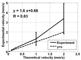
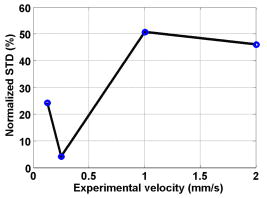
1. Introduction

Blood flow in an organ or tissues through capillaries represents an important factor for diagnosing pathological conditions, including heart failure,¹ liver cirrhosis,² and pancreatitis,³ and for evaluating the physiological condition, such as in renal transplants.⁴ Moreover, antiangiogenesis therapies for tumors have recently received wide attention in animal models used in preclinical research.^{5, 6} Treatment effects can be evaluated by longitudinal observation of tumor angiogenesis, which can be achieved by measuring the capillary flow in the tumor.^{7, 8} The flow rate in a considerable small region of interest (ROI) is commonly measured by monitoring the concentrations of exogenous indicators, which is also known as the contrast-specific measurement method.^{9, 10, 11} Recently, we have successfully developed contrast-specific methods for photoacoustic measurements of flow using gold nanorods as the contrast agent.^{12, 13, 14, 15} Although these methods have been shown to be effective, they are designed for measuring flows in large vessels, where the ROI is inside the vessel. In this work, we extend the method to vessels smaller than the photoacoustic sample volume using a high-frame-rate photoacoustic imaging system. One major advantage of such a 2-D photoacoustic flow measurement system is that it provides both anatomical and flow information.

Contrast-specific flow measurements have been developed using various imaging modalities, such as computed tomography,^{2, 3, 16} magnetic resonance imaging,^{17, 18} and ultrasound.¹⁹ Contrast agents are used as flow indicators, with their dilution monitored as a function of time. In general, contrast agents are materials that are injected into the human body to enhance the signal-to-noise ratio (SNR) of blood vessels in the ROI. Although concentration is the parameter of interest, most contrast-specific methods measure the signal intensity, implicitly assuming that the intensity is linearly proportional to the concentration.^{17, 19} The measured signal intensity over time is also known as the time-intensity curve (TIC). The flow rate is determined based on the indicator-dilution theory,^{20, 21, 22} which typically employs a mixing chamber that relates the two TICs obtained at the inflow and outflow of the mixing chamber. The mixing chamber is often modeled as a linear and time-invariant (LTI) system, and therefore the relation between the input and output of the mixing chamber can be described by a transfer function as a wash-out analysis.²³ The transfer function is approximated as an exponential function with a time constant determined by the flow rate. Therefore, given both the input and output TICs, deconvolution can be applied to estimate the transfer function, from which the flow rate can be determined.²⁴ The applicability of the deconvolution-based method is determined by the validity of the LTI system model and the accuracy of deconvolution.²⁴

Wash-in flow estimation methods have been proposed that overcome the difficulties associated with deconvolution-based methods.^{15, 19, 25} This method requires the concentration of the contrast agent to be reduced by “destroying” indicators in the ROI. In ultrasonic imaging, for example, a microbubble-based contrast agent can be destroyed by irradiation with acoustic pulses of sufficient energy,^{25, 26} with the subsequent temporal changes in the concentration determined by the replenishment rate of the contrast agent (i.e., new microbubbles flowing into the ROI). This replenishment process is related to the local flow rate.¹⁵ Because deconvolution is not required, the wash-in method is generally more stable and accurate.

We have previously developed wash-in flow measurements for photoacoustic imaging^{14, 15} using gold nanorods as the photoacoustic contrast agent. Gold nanorods are biomedically compatible materials that offer a strong photoacoustic response in the visible to near-infrared region.²⁷ The wavelength at which a nanorod exhibits peak optical absorption is determined by its aspect ratio (defined as the length of the major axis divided by that of the minor axis). The shape of a nanorod can be altered by laser pulses with sufficient energy, which is known as the nanorod-to-nanosphere shape transition.²⁸ The laser-induced shape transition of gold nanorods leads to a reduction of the aspect ratio (often being transformed into nanospheres) and causes a downshift of the absorption peak. In practice, the nanorods are not destroyed, but instead their shapes are changed, which effectively reduces the concentration of the nanorods with the original aspect ratio, and the associated shift in the peak absorption wavelength is monitored. The wash-in flow measurements used in ultrasonic imaging are still applicable.

The purpose of this work is to extend the previously proposed method from flow estimation from a single ROI to 2-D mean flow velocity measurements. Achieving this requires a 2-D photoacoustic imaging system with an adequate frame rate, the design and construction of which is also described here. The accuracy of flow rate measurements made by applying this system to flow phantoms is also reported.

This work is organized as follows. The principles of flow rate measurement based on the time-intensity method are described in Sec. 2. Section 3 describes the high-frame-rate imaging system and the experimental apparatus of the flow rate measurement. Section 4 describes the measurement results from flow phantoms. Section 5 discusses the results and the range of flow rates measurable by this system, and conclusions are drawn in Sec. 6.

2. Principles of Photoacoustic Wash-in Flow Measurement

The method used to estimate the flow rate consists of both the destruction (i.e., depletion) and the replenishment (i.e., wash-in) of the nanorods. Laser pulses with a sufficiently high energy are used to cause rod-to-sphere shape transitions, and also to monitor the reduced concentration of gold nanorods in the ROI. The process is illustrated in more detail in Fig. 1 . A steady state is first reached before the application of laser pulses $(t < t_{0})$ after the injection of the gold nanorods. A laser pulse transforms gold nanorods into nanorods with a smaller aspect ratio (possibly into nanospheres) at $t = t_{0 -}$ , and the detected photoacoustic-signal intensity is reduced $(t = t_{0 +})$ . After that, new nanorods (without shape transitions) flow into the ROI at a rate determined by the flow rate $(t_{0} < t < t_{1})$ , and the concentration of gold nanorods with the original aspect ratio increases in the ROI. Another laser pulse irradiates after a pulse repetition interval (PRI) and causes another period of destruction and the following replenishment of the gold nanorods. After several periods of the destruction-replenishment process, the concentration of nanorods in the ROI will reach a steady state if the number of incoming new nanorods approximates that of the destroyed nanorods.

Fig. 1

Illustration in the wash-in process (top) and its corresponding concentration curve (bottom). After infusion, the concentration of gold nanorods reaches an equilibrium (I). The laser-induced shape transitions result in the nanorods inside the laser beam being transformed into nanospheres (or rods with a smaller aspect ratio) after each laser pulse (II and IV). New nanorods flow at a certain rate into the region without laser irradiationed (III and V).

The TIC measured in this period of time can be used to calculate the flow rate by fitting it to a curve derived from the replenishment model. The model used was adapted and modified from our previous work.¹⁵ Assuming that the laser beam is much larger than the diameter of the capillaries inside a flow region and that the beam profile of the ultrasound transducer along the $y$ axis is $u (y)$ , the effective concentration measured by this transducer is

Eq. 1

n^{'} (t) = \frac{\int n (y; t) u (y) d y}{\int u (y) d y} = \int n (y; t) \hat{u} (y) d y,

where

\hat{u} (y) = u (y) ∕ \int u (y_{0}) d y_{0}

, and

n (y; t)

denotes the concentration of gold nanorods in the vessel as a function of position

(y)

and time

(t)

, the initial value of which is

n_{0}

. A sequence of laser pulses with a fixed PRI is applied from

t = t_{0}

. To derive the model for TICs, the interlacing destruction by laser energy and replenishment of flow should be assessed respectively. The short periods between

t = {(t_{0} + k ∙ PRI)}^{-}

and

t = {(t_{0} + k ∙ PRI)}^{+}

, i.e., laser pulse duration, are called the destruction phases, where

k

is the pulse index. The replenishment phases occur between

t = {(t_{0} + k ∙ PRI)}^{+}

and

t = {[t_{0} + (k + 1) ∙ PRI]}^{-}

, i.e., a PRI. The superscripts + and − in the subscripts represent “soon after” and “immediately before,” respectively.

In the replenishment phase, predicting $n (y; t)$ for $t > t_{0}$ based on $n (y; t_{0})$ is required to estimate flow parameters, for which the initial condition is $n (y; t_{0}) = n_{0} - n_{0} l (y)$ , where $l (y)$ denotes the shape of the laser beam along the $y$ axis and is typically a low-pass function of $y$ . Assuming that the flow system is linear and shift invariant gives

Eq. 2

n (y; t) = \int g (y - y_{0}; t, t_{0}) n (y_{0}; t_{0}) d y_{0} = n_{0} - n_{0} g (y; t, t_{0}) \otimes l (y),

where ⊗ denotes convolution (along

y

), and

g (y - y_{0}; t, t_{0})

, i.e., the transfer function, is the

n (y; t)

corresponding to

n (y; t_{0}) = δ (y - y_{0})

, where

δ (y)

is the Dirac delta function. From Eqs. 1, 2 we can obtain

Eq. 3

n^{'} (t) = n_{0} {1 - h [v (t - t_{0})]},

where

Eq. 4

h [v (t - t_{0})] = \int [g (y; t, t_{0}) \otimes l (y)] u^{'} (y) d y .

According to the random-walk model,²⁹ the density of label, i.e., nanoparticles, along the flow direction

x

after a bolus injection can be represented as

F (x, σ) = (1 ∕ σ \sqrt{2 π}) \exp [- {(x - \bar{x})}^{2} ∕ 2 σ^{2}]

, where

σ

and

\bar{x}

denote the random variable and the distance after the injection, respectively. In this case, the bolus injection, which is produced by the rapid laser destruction, is determined at

t = t_{0}

, and

σ = \sqrt{2 D (t - t_{0})}

at the central position of

\bar{x} = v (t - t_{0})

. Therefore,

Eq. 5

g (y - y_{0}; t, t_{0}) = \frac{1}{\sqrt{4 π D (t - t_{0})}} \exp {- \frac{{[y - y_{0} - v (t - t_{0})]}^{2}}{4 D (t - t_{0})}},

where

D

is the dispersion coefficient representing the randomness.^{29, 30} Assuming that both the laser and the ultrasound beam profile are Gaussian distributed in

y

[i.e.,

u^{'} (y) = \exp (- y^{2} ∕ σ_{u}^{2}) ∕ \sqrt{π σ_{u}^{2}}

and

l (y) = l_{0} \exp (- y^{2} ∕ σ_{l}^{2}) ∕ \sqrt{π σ_{l}^{2}}

, where

σ_{u}

and

σ_{l}

are standard deviations of the ultrasound and the laser beam profile, respectively], Eq. 4 can be solved as

Eq. 6

h [v (t - t_{0})] = \frac{l_{0}}{{π [4 D (t - t_{0}) + σ_{u}^{2} + σ_{l}^{2}]}^{1 ∕ 2}} \exp {- \frac{{[v (t - t_{0})]}^{2}}{4 D (t - t_{0}) + σ_{u}^{2} + σ_{l}^{2}}} .

A reasonable approach to curve fit

h [v (t - t_{0})]

is to use

Eq. 7

\hat{h} (k) = h (0) \exp (- λ k),

where

λ

is a model parameter, and

k

is the variable in the fitted curve. It represents the distance after a period of time

(t - t_{0})

. Under this condition, Eq. 3 can be rewritten as

Eq. 8

n^{'} (t) ≅ n_{0} {1 - c \exp [- λ v (t - t_{0})]} = n_{0} {1 - c \exp [- β (t - t_{0})]},

where

c

and

β

are model parameters, and

β

is proportional to the flow rate

v

. This equation describes the concentration change as a function of time in the replenishment phase. Therefore, the effects of the replenishment phases between each laser pulse firing can be estimated according to Eq. 8,

Eq. 9

{1 - n^{'} (t - t_{0}) ∣}_{t = {(t_{0} + k ∙ PRI)}^{+}} ∕ n_{0} ≅ c {\exp [- β (t - t_{0})] ∣}_{t = {(t_{0} + k ∙ PRI)}^{+}},

Eq. 10

{1 - n^{'} (t - t_{0}) ∣}_{t = {[t_{0} + (k + 1) ∙ PRI]}^{-}} ∕ n_{0} ≅ c {\exp [- β (t - t_{0})] ∣}_{t = {[t_{0} + (k + 1) ∙ PRI]}^{-}} .

The concentration of gold nanorods in the replenishment phase can be described as:

Eq. 11

{1 - n^{'} (t - t_{0}) ∣}_{t = {[t_{0} + (k + 1) ∙ PRI]}^{-}} ∕ n_{0} ≅ \exp (- β ∙ PRI) [{1 - n^{'} (t - t_{0}) ∣}_{t = {(t_{0} + k ∙ PRI)}^{+}} ∕ n_{0}] .

On the other hand, in the destruction phases, it is noticeable that the replenishment during the destruction phase is negligible because the pulse duration is on the order of nanoseconds and is much smaller than the length of the PRI. In these periods, destruction mainly dominates the behavior of the concentration of nanorods. The concentration decreases asymptotically to a constant level and can be expressed as:

Eq. 12

{n^{'} (t - t_{0}) ∣}_{t = {(t_{0} + k ∙ PRI)}^{-}} ≅ (n_{0} - n_{\infty}) r^{k} + n_{\infty} for k = 0, 1, 2, \dots,

where

r < 1

is the survival rate, which indicates the remained nanorods after one laser pulse.

n_{\infty}

is the baseline concentration. And the concentration of the gold nanorods after each laser pulse can be expressed as:

Eq. 13

{n^{'} (t - t_{0}) ∣}_{t = {(t_{0} + k ∙ PRI)}^{+}} ≅ r {n^{'} (t - t_{0}) ∣}_{t = {(t_{0} + k ∙ PRI)}^{-}} .

Finally, we can obtain the concentration of the nanorods by combining the destruction phase in Eq. 13 with the replenishment phase in Eq. 11:

Eq. 14

{1 - n^{'} (t - t_{0}) ∣}_{t = {[t_{0} + (k + 1) ∙ PRI]}^{-}} ∕ n_{0} ≅ \exp (- β ∙ PRI) [1 - r {n^{'} (t - t_{0}) ∣}_{t = {(t_{0} + k ∙ PRI)}^{-}} ∕ n_{0}] .

Let

n^{″} (k) = {n^{'} (t - t_{0}) ∣}_{t = {(t_{0} + k ∙ PRI)}^{-}} ∕ n_{0}

, then we can have

Eq. 15

n^{″} (k + 1) = 1 - [1 - r n^{″} (k)] s,

where

s = \exp (- β ∙ PRI)

, and solving Eq. 15 with

n^{″} (0) = 1

leads to

Eq. 16

n^{″} (k) = (\frac{1 - s}{1 - r s}) + [1 - (\frac{1 - s}{1 - r s})] {(r s)}^{k} .

Equation 16 indicates that the concentration of gold nanorods decreases exponentially to a constant value determined by the flow velocity and the laser pulse energy. Let

n_{\infty}^{″} = 1 - s ∕ 1 - r s

and

w = r s

, then we can obtain a fitting model for the measured TIC:

Eq. 17

n^{″} (k) = n_{\infty}^{″} + (1 - n_{\infty}^{″}) w^{k} .

Finally, the mean velocity can be obtained from the value of the fitted parameter:

Eq. 18

β = v ∙ λ = - \log [1 - (1 - w) n_{\infty}^{″}] ∕ PRI .

According to Wei, ¹⁹

λ

is inversely proportional to the width of the detection region (i.e., the width of laser beam

E = 1 ∕ λ

). Therefore, the flow rate can be calculated from the fitted parameter according to

Eq. 19

v = β ∙ E .

3. Experimental Setup

3.1.

High-Frame-Rate Photoacoustic Imaging System

The photoacoustic technique combines laser irradiation and acoustic detection. It offers advantages of both a higher optical contrast than conventional ultrasound and a better penetration depth as compared with all-optical imaging techniques such as microabsorption spectrometry and dark-field microscopy. The capabilities of photoacoustic imaging have been demonstrated in many applications, including functional imaging of rat brain,³¹ breast tumor detection,³² and molecular imaging.³³ Nanoparticles have also been used as contrast agents and molecular probes.^{34, 35} Generally, when a tissue is irradiated by an incident laser pulse, absorption of the laser energy leads to a rapid temperature rise, thermal expansion, and the concomitant generation of broadband ultrasound waves.³⁶ These waves can be used to estimate optical properties (i.e., the optical absorption) of the tissue.

According to the wash-in flow measurement model described in Sec. 2, flow rate measurements require the optical absorption of nanorods to be monitored over a considerable period of time. During the replenishment period, absorption changes have to be measured over a short time interval (i.e., requiring a high sampling rate). We have previously demonstrated that a sampling rate of $15 Hz$ allows flow velocities from $0.35 to 2.8 mm ∕ s$ to be measured in a single sample volume.¹⁴

The 2-D photoacoustic imaging system used in this study employed an array transducer instead of a single-crystal transducer to increase the frame rate by allowing data to be acquired simultaneously from multiple channels. This high-frame-rate photoacoustic imaging system consisted of a fiber laser system, an ultrasonic digital phased array system (DiPhAS), which is often used in research applications, and a custom-design photoacoustic probe, as shown in Fig. 2 . A Q-switched Nd:YAG laser (LS-2132U, Lotis TII, Belarus) operating at $1064 nm$ with a pulse duration of $8 ns$ was used for laser irradiation. The $5 - mm$ -diam beam from this laser was split and guided onto two multimode fiber light guides (LG-L30-6-H-1500-F-1, Taiwan Fiber Optics, Taiwan) using a half-reflectance beamsplitter (BS1-1064-50, CVI, NM). The output beams from the light guides were then focused by two cylindrical lenses positioned $25 mm$ from the light-guide surfaces, resulting in two irradiated zones of $30 \times 0.8 mm$ . Both the light guides and the focusing lenses were mounted on a custom-design holder as part of the photoacoustic probe for confocal alignment. A motorized lens wheel (FW102, Thorlabs, New Jersey) placed between the laser and the beamsplitter was used to switch the laser energy.

Fig. 2

(a) Schematic of the high-frame-rate photoacoustic imaging system that includes a fiber laser system, a DiPhAS, and custom-made photoacoustic probe. (b) Custom-made photoacoustic probe. The output beams from the light guides are focused by two cylindrical lenses positioned $25 mm$ from the light-guide surfaces. The focused laser beam and the ultrasound detection area are aligned confocally.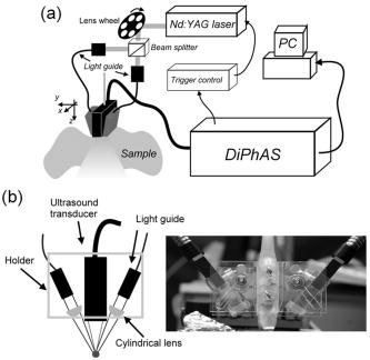

Acoustic waves induced in the irradiated volume were detected by a 128-channel ultrasonic linear array (L6, Sound Technology, Pennsylvania) that was also confocally mounted between the two light guides in the photoacoustic probe, as shown in Fig. 2b. The transducer elements had a pitch of $0.3 mm$ , a $5 - mm$ elevational width, and a center frequency of $5 MHz$ with an 82% bandwidth. Reflecting foil (Ho Yan Tape, Taiwan) with a thickness of $9 μ m$ was attached to the surface of the transducer to block backscattered laser irradiation from reaching the transducer surface. The DiPhAS was employed to amplify and digitize the detected rf array signals. It contained 64 transmitting and receiving channels and high-speed multiplexers to allow the use of a transducer array with up to 192 channels, although in this study the multiplexers were not used. The rf signals from the 64 transducer elements sent to the receiver were amplified by up to $80 dB$ and then digitized by analog-to-digital converters with $12 - bit$ precision. The data were sampled at $40 Msamples ∕ s$ , and the on-board memory allowed 512 data samples per channel to be stored before they were transferred to a personal computer (PC). The DiPhAS allowed array data from 64 channels to be simultaneously acquired and transferred every $4 ms$ , giving a frame rate of up to $250 Hz$ . The raw rf data were transferred through a high-speed digital I/Q card (PCI-7300A, ADlink, Taiwan) to the PC, and dynamic focusing and image reconstruction were performed off-line. The DiPhAS and laser were synchronized using a programmable logic device (EPM3064A, Altera, California), with the laser triggered by the DiPhAS. The actual frame rate of the system was limited to $15 Hz$ due to the maximum PRF of the laser that we used.

In this study, 2-D photoacoustic images captured from the same flow region over the replenishment period were used to evaluate the concentration change of gold nanorods. ROIs were chosen to include the flow area of interest, such as capillaries or organs. The mean photoacoustic intensities in these ROIs were calculated at each time step as a data point in the TIC. Therefore, there is a tradeoff between the SNR and the size of the ROI (which determines the spatial resolution).

3.2.

Flow Phantom

Figure 3 shows a schematic diagram of the flow measurement setup. A sample was made of chicken breast tissue, in which polyethylene tubing (Intramedic™ 427411, Sparks, Maryland) with a inner diameter of $580 μ m$ was embedded at a depth of $2 mm$ . A volume of $1 ml$ of human blood and $55 μ l$ of gold nanorods with an absorption peak at $985 nm$ at a concentration of $3.6 nM$ were mixed and injected into the tubing with a $1 - ml$ standard syringe. The absorption peak of the nanorods was measured using a spectrophotometer (V-570, Jasco, Japan). The syringe was controlled by an infusion pump (KDS 100, Montreal, Canada) to create mean flow velocities ranging from $0.125 to 2 mm ∕ s$ . The theoretical flow velocity is the mean value of the entire flow region. It was calculated from the pumping rate of the infusion pump with the cross sectional area size of flow region (i.e., the tubing). Before these experiments, the pumping rate has been tested by measuring the weight of the pumped water. The photoacoustic probe was positioned $13 mm$ above the tube, and cross sectional images were captured. TICs were achieved by summing the photoacoustic intensities from within a $0.6 \times 1.2 - mm$ ROI $(8 \times 4 pixels$ in the $z$ and $x$ axes, respectively) at each time point.

Fig. 3

Experimental setup of the flow phantom, in which the flow rate was controlled by the infusion pump with a syringe. The tubing was placed inside the chicken breast tissue to simulate tissue microcirculation. The flow velocities ranged from $0.125 to 2 mm ∕ s$ .

A pilot experiment indicated that applying laser irradiation at energy densities of $82.4 mJ ∕ {cm}^{2}$ was suitable for the destruction of the nanorods in the tube. Figure 4 shows that the image intensity decayed within $4 s$ . Figure 5 shows the visible-to-infrared spectra of the nanorods before and after the applications of the destruction pulses as measured using the spectrophotometer, with the gray rectangle highlighting the large absorbance difference at $1064 nm$ (the wavelength of the laser irradiation). Figure 6 demonstrates the linearity of the relation between the concentration of the nanorods and the photoacoustic intensities before the flow experiments (for an energy density of $6.45 mJ ∕ {cm}^{2}$ ), and thus the validity of monitoring nanorod concentration by measuring photoacoustic signals.

Fig. 4

Image intensities measured with the laser energy of $82.4 mJ ∕ {cm}^{2}$ . The intensity rapidly decayed to 90% within 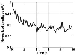$4 s$ .

Fig. 5

Spectra of nanorods before (solid line) and after (dashed line) the laser-induced shape transition. The gray rectangle indicates the wavelength of the laser irradiation (around $1064 nm$ ).

Fig. 6

Measured photoacoustic intensity as a function of nanorod concentration for laser energy of $6.45 mJ ∕ {cm}^{2}$ .

4. Experimental Results

Figure 7 shows focused cross sectional images of the flow phantom. In this figure, the positions of the chicken breast tissue and the tubing show consistent with their location. The tubing is at a depth of $2 mm$ from the chicken breast surface, a fact that the laser energy irradiates the tubing after propagating through light scattering and absorbing biological tissue. In this case, the destruction of the gold nanorods from the outer tissue sample becomes difficult, since the laser intensity decays along the propagation depth due to the light attenuation. Images captured during the measurement $(t = 0 to 16.5 s)$ are shown in Figs. 8a, 8b, 8c , displayed with a dynamic range of $- 10 dB$ . These images display a depth of $2.5 mm$ and a width of $5 mm$ , and were normalized by subtracting the background image captured without gold nanorods. Therefore, these images show only the photoacoustic signals from the nanorods. The laser energy was set at $82.4 mJ ∕ {cm}^{2}$ (i.e., at $t = 0 s$ ). It is clear that the image intensity decreases with time, indicating that the gold nanorods inside the tube underwent shape changes due to the strong incident laser energy that reduced the optical absorption at the laser wavelength. A steady state was reached after continuous laser irradiation at the same energy level for $16 s$ , at which point the number of nanorods that underwent shape transition was roughly the same as the number of new nanorods flowing into the ROI. A square region with a size of $0.6 \times 1.2 mm$ was selected as the ROI, as indicated by the dashed box in Fig. 8a. The mean image intensities within the ROI were summed to create the TIC. Figure 9 shows the normalized TICs measured at flow rates of 0.125, 0.25, 1, and $2 mm ∕ s$ , which clearly indicate that the replenishment rate of the nanorods increases with the flow rate, as described by Eq. 17.

Fig. 7

Chicken breast image. The tubing with an inner diameter of $580 μ m$ was placed at a depth of $2 mm$ from the tissue surface. The displayed dynamic range is 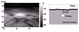$45 dB$ .

Fig. 8

Images captured at different times at a flow rate of $0.125 mm ∕ s$ . The displayed dynamic range is $10 dB$ . Note that these images were normalized by subtracting the background image captured without gold nanorods.

Fig. 9

Normalized TICs (markers) and their corresponding fitted curves (lines) at flow rates of 0.125, 0.25, 1, and $2 mm ∕ s$ , respectively.

The TICs were then calculated by fitting, which was performed using MATLAB (The MathWorks, Natick, Massachusetts). The TICs were measured five times in each case, from which mean and standard deviation (STD) values were calculated. In Eq. 18, flow rate $v$ is proportional to the product of fitting parameter $β$ (i.e., rate constant) and the width of irradiated volume $E$ . Figure 10 shows the mean flow rate calculated for irradiated zones with widths ranging from $0.2 to 1.0 mm$ . The results calculated with a large $E$ (i.e., a broad irradiated zone along the $y$ axis) are overestimations, whereas a small $E$ results in underestimations of the flow velocity. It is clear from the figure that using $E = 0.5 mm$ gives the best agreement with the theoretical flow rate. However, the width of the irradiated volume of this system is $0.8 mm$ (which was measured by using a knife-edge method).

Fig. 10

Estimation results of the flow rate for $E$ values from $0.2 to 1 mm$ .

A comparison between the experimental results using $E = 0.8 mm$ and the actual flow velocities is shown in Fig. 11 . Because the ROI covers nearly the entire cross section of the tube, the measured results can be viewed as the mean flow velocity inside the sample volume. It is obvious that most of the flow velocities are overestimated. The linear regression curve between the measured velocities $(y)$ and the actual velocities $(x)$ is described by $y = 1.68 x - 0.12$ , which indicates that the measured flow velocity is higher than the actual one. The correlation coefficient between the measured flow velocities and their linear regression fit was 0.83. Figure 11 also shows that the STDs increase with the mean values, with Fig. 12 plotting the normalized STD-to-mean ratios (the average value is 31.3%). This relationship may be attributable to the SNR of TICs. In high flow velocities, replenishment becomes more effective, which means that the steady state (in which the number of incoming new nanorods approximates to that of the destroyed nanorods) is easier to approach, as shown in Fig. 9. Therefore, fitting such low contrast curves without sufficient SNR leads to measurement errors. This problem can be solved if a larger ROI is chosen to increase the SNR.

Fig. 11

Flow rate estimation results (solid line), its linear fit (dashed), and the ideal curve (dotted line) for an irradiated zone with a width of $0.8 mm$ .

Fig. 12

Normalized STD versus the flow velocity. The average value is 31.3%.

5. Discussion

The results presented here show that the wash-in flow estimation method can be implemented utilizing images captured by a high-frame-rate photoacoustic imaging system. However, two issues need to be addressed before making in-vivo measurements. First, our experiments were conducted with a measured laser beam width. However, the width of the irradiated zone in the tissue is difficult to evaluate when the laser pulse propagates through a strongly scattering medium, and an incorrect width leads to measurement errors, as shown in Fig. 10. Therefore, the difference between the assumed and actual width is a critical problem in this method if absolute measurements are required. Nonetheless, relative measurements can be made even in the presence of errors in $E$ . Second, the measurable range of the flow rate is determined by both the frame rate (i.e., sampling rate) and the width of the irradiated zone in the ROI. There is therefore a tradeoff between the elevational resolution (i.e., the resolution along the axis perpendicular to the cross sectional image) and the measurable flow rate. On the other hand, actual flow rates ranging from $0.5 to 10 mm ∕ s$ in capillaries smaller than $200 μ m$ have been verified using intravital microscopy.²⁸ Therefore, such applications of this method require a system with a broad sampling range. In addition, preclinical investigations with small-animal models require a better spatial resolution for identifying their anatomic structures.

The rate constant is defined as the ratio of the flow velocity to the width of the irradiated zone, and represents the replenishment rate inside the irradiated volume (see Fig. 1). A large rate constant means that the concentration of new nanoparticles inside the irradiated zone rapidly reaches a steady state. Therefore, either increasing the flow velocity or decreasing the width of the irradiated zone increases the rate constant. Based on this principle, the flow velocity can be determined from the width of the irradiated zone and the sampling rate.

To investigate the relation between the rate constant $β$ and the sampling rate, TICs were calculated for various rate constants ranging from $0.2 to 10 ∕ s$ using Eq. 16. The simulated TICs were sampled at rates ranging from $1 to 50 samples ∕ s$ . These TICs were curve fitted for rate-constant estimation (as the last step in flow estimation). Comparisons between the measured rate constants with the predetermined values are presented in Fig. 13 . In this figure, most of the resulting ratios are more than unity, meaning that the measured rate constant is 10 to 20% higher than the determined one. This could be a possible reason of the overestimations shown in Fig. 11. On the other hand, it is also noticeable that the resulting ratios are less than unity when the sampling rate is insufficient, meaning that the measured flow rate is lower than the determined one. This may be due to a high-flow velocity in an irradiated zone, resulting in a large rate constant and thus a short replenishment period. With an irradiated zone of constant width and a fixed frame rate, underestimation is worse when the flow velocity is higher (i.e., $higher β$ ). In Fig. 13, the system frame rate of $15 Hz$ is indicated by the vertical dashed line. The flow velocity corresponding to rate constants of $0.2 ∕ s$ , $1 ∕ s$ , and $5 ∕ s$ are 0.16, 0.8, and $4 mm ∕ s$ , respectively (assuming an irradiation width of $0.8 mm$ ).

Fig. 13

Ratio of the measured $β$ to the predetermined $β$ from numerical simulations. The frame rate of the current system (i.e., $15 Hz$ ) is indicated by the vertical dashed line.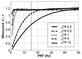

In our previous work, we also reported a two-energy wash-in flow estimation method. This method contains a sequence of laser pulses to destroy gold nanorods, and a following sequence with lower laser energy to monitor the replenishment.¹⁵ However, lower laser energy propagated through turbid biological tissues cannot provide sufficient SNR for the replenishment measurement. Therefore, in strong scattering and absorbing tissue, it is much easier to achieve the flow estimation method in single energy than that in double energy.

Although color Doppler techniques have been routinely used in diagnostic ultrasound, there have been no reliable flow estimation methods available for photoacoustic imaging other than the proposed method in our study. It is therefore the purpose of this study to demonstrate the feasibility of our approach. Current color Doppler techniques estimate blood flow velocities by calculating the phase of the autocorrelation function of the baseband Doppler signals.^{37, 38} However, such phase-sensitive techniques are not applicable in photoacoustic imaging. In addition, the phase measurement is sensitive to noise and susceptible to tissue motion. Particularly for low velocity flows, design of the clutter filters becomes challenging, if not impossible.³⁹ Note that the proposed method is less affected by noise because contrast agents (gold nanoparticles) are used. The estimation can also be performed more reliably because the data are collected over a longer period of time and signal averaging is generally applied.

6. Conclusions

We experimentally demonstrate the feasibility of nanorod-based flow measurement based on a high-frame-rate photoacoustic imaging system, which currently has a frame rate up to $15 Hz$ . The linearity between the nanorod concentration and photoacoustic intensities is verified. The results of the flow experiments show that flow velocities ranging from $0.125 to 2 mm ∕ s$ can be measured, with an average normalized STD of 31.3%. The measurable flow rate of this method is limited by the PRF of the laser system. The feasibility of in-vivo studies is also been discussed. To apply this flow measurement method to preclinical research involving small-animal models, one future direction is to build a photoacoustic imaging system equipped with a transducer array operating at a higher frequency (to improve the imaging spatial resolution), and a laser with a higher PRF (to provide a high frame rate).

Acknowledgments

The authors gratefully acknowledge Chung-Ren Chris Wang and Kuei Chen Pao for helpful comments and providing the gold nanorods used in this work. This work was financially supported by the National Science Council under grants NSC-94-2213-E-002-115 and NSC-94-2120-M-002-004, and by the National Taiwan University Nano Center for Science and Technology and National Health Research Institutes.

References

1.

C. J. Hogan, M. L. Hess, K. R. Ward, and C. Gennings, “The utility of microvascular perfusion assessment in heart failure: a pilot study,” J. Card. Fail, 11 713 –719 (2005). 1071-9164 Google Scholar

2.

C. Weidekamm, M. Cejna, L. Kramer, M. Peck-Radosavljevic, and T. R. Bader, “Effects of TIPS on liver perfusion measured by dynamic CT,” AJR, Am. J. Roentgenol., 184 505 –510 (2005). 0361-803X Google Scholar

3.

P. E. Bize, A. Platon, C. D. Becker, and P. A. Poletti, “Perfusion measurement in acute pancreatitis using dynamic perfusion MDCT,” AJR, Am. J. Roentgenol., 186 114 –118 (2006). https://doi.org/10.2214/AJR.04.1416 0361-803X Google Scholar

4.

T. Scholbach, E. Girelli, and J. Scholbach, “Tissue pulsatility index: a new parameter to evaluate renal transplant perfusion,” Transplantation, 81 751 –755 (2006). https://doi.org/10.1097/01.tp.0000201928.04266.d2 0041-1337 Google Scholar

5.

P. Schulz, A. Scholz, A. Rexin, P. Hauff, M. Schirner, B. Wiedenmann, K. Detjen, and S. Rosewicz, “Reconstitution of p16INK4a in an orthotopic pancreatic mouse model inhibits tumor growth and angiogenesis,” Gastroenterology, 130 A35 –A35 (2006). 0016-5085 Google Scholar

6.

T. Aikawa, J. Gunn, S. M. Spong, S. J. Klaus, and M. Korc, “Connective tissue growth factor-specific antibody attenuates tumor growth, metastasis, and angiogenesis in an orthotopic mouse model of pancreatic cancer,” Mol. Cancer Ther., 5 1108 –1116 (2006). Google Scholar

7.

N. S. Akella, D. B. Twieg, T. Mikkelsen, F. H. Hochberg, S. Grossman, G. A. Cloud, and L. B. Nabors, “Assessment of brain tumor angiogenesis inhibitors using perfusion magnetic resonance imaging: quality and analysis results of a phase I trial,” J. Magn. Reson Imaging, 20 913 –922 (2004). 1053-1807 Google Scholar

8.

D. Maya, F. H. Edna, and D. Hadassa, “The application of NMR in tumor angiogenesis research,” Prog. Nucl. Magn. Reson. Spectrosc., 49 27 –44 (2006). 0079-6505 Google Scholar

9.

T. Holscher, W. Wilkening, B. Draganski, S. H. Meves, J. Eyding, H. Voit, U. Bogdahn, H. Przuntek, and T. Postert, “Transcranial ultrasound brain perfusion assessment with a contrast agent-specific imaging mode: results of a two-center trial,” Stroke, 36 2283 –2285 (2005). https://doi.org/10.1161/01.STR.0000179038.63109.b0 0039-2499 Google Scholar

10.

T. Holscher, T. Postert, S. Meves, T. Thies, H. Ermert, U. Bogdahn, and W. Wilkening, “Assessment of brain perfusion with echo contrast specific imaging modes and Optison,” Acad. Radiol., 9 S386 –S388 (2002). 1076-6332 Google Scholar

11.

C. Pohl, K. Tiemann, T. Schlosser, and H. Becher, “Stimulated acoustic emission detected by transcranial color Doppler ultrasound: a contrast-specific phenomenon useful for the detection of cerebral tissue perfusion,” Stroke, 31 1661 –1666 (2000). 0039-2499 Google Scholar

12.

P. C. Li, C. W. Wei, C. K. Liao, H. C. Tseng, Y. P. Lin, and C. C. Chen, “Time-intensity based optoacoustic flow measurements with gold nanoparticles,” Proc. SPIE, 5697 63 –72 (2005). https://doi.org/10.1117/12.591106 0277-786X Google Scholar

13.

C. W. Wei, C. K. Liao, H. C. Tseng, Y. P. Lin, C. C. Chen, and P. C. Li, “Photoacoustic flow measurements with gold nanoparticles,” IEEE Trans. Ultrason. Ferroelectr. Freq. Control, 53 1955 –1959 (2006). https://doi.org/10.1109/TUFFC.2006.128 0885-3010 Google Scholar

14.

P. C. Li, S. W. Huang, C. W. Wei, Y. C. Chiou, C. D. Chen, and C. R. Wang, “Photoacoustic flow measurements by use of laser-induced shape transitions of gold nanorods,” Opt. Lett., 30 3341 –3343 (2005). https://doi.org/10.1364/OL.30.003341 0146-9592 Google Scholar

15.

P. C. Li, S. W. Huang, C. W. Wei, and C. R. C. Wang, “Destruction-mode optoacoustic flow measurements with gold nanorods,” Proc.-IEEE Ultrason. Symp., 2 1348 –1351 (2005). 1051-0117 Google Scholar

16.

G. J. Hunter, H. M. Silvennoinen, L. M. Hamberg, W. J. Koroshetz, F. S. Buonanno, L. H. Schwamm, G. A. Rordorf, and R. G. Gonzalez, “Whole-brain CT perfusion measurement of perfused cerebral blood volume in acute ischemic stroke: probability curve for regional infarction,” Radiology, 227 725 –730 (2003). https://doi.org/10.1148/radiol.2273012169 0033-8419 Google Scholar

17.

E. Johansson, L. E. Olsson, S. Mansson, J. S. Petersson, K. Golman, F. Stahlberg, and R. Wirestam, “Perfusion assessment with bolus differentiation: a technique applicable to hyperpolarized tracers,” Magn. Reson. Med., 52 1043 –1051 (2004). https://doi.org/10.1002/mrm.20247 0740-3194 Google Scholar

18.

L. Bentzen, M. R. Horsman, P. Daugaard, and R. J. Maxwell, “Non-invasive tumour blood perfusion measurement by 2H magnetic resonance,” NMR Biomed., 13 429 –437 (2000). https://doi.org/10.1002/1099-1492(200012)13:8<429::AID-NBM663>3.0.CO;2-K 0952-3480 Google Scholar

19.

K. Wei, A. R. Jayaweera, S. Firoozan, A. Linka, D. M. Skyba, and S. Kaul, “Quantification of myocardial blood flow with ultrasound-induced destruction of microbubbles administered as a constant venous infusion,” Circulation, 97 473 –483 (1998). 0009-7322 Google Scholar

20.

X. C. Chen, K. Q. Schwarz, D. Phillips, S. D. Steinmetz, and R. Schlief, “A mathematical model for the assessment of hemodynamic parameters using quantitative contrast echocardiography,” IEEE Trans. Biomed. Eng., 45 754 –765 (1998). https://doi.org/10.1109/10.678610 0018-9294 Google Scholar

21.

L. Claassen, G. Seidel, and C. Algermissen, “Quantification of flow rates using harmonic grey-scale imaging and an ultrasonic contrast agent: an in vitro and in vivo study,” Ultrasound Med. Biol., 27 83 –88 (2001). https://doi.org/10.1016/S0301-5629(00)00324-0 0301-5629 Google Scholar

22.

P. A. Heidenreich, J. G. Wiencek, J. G. Zaroff, S. Aronson, L. J. Segil, P. V. Harper, and S. B. Feinstein, “In vitro calculation of flow by use of contrast ultrasonography,” J. Am. Soc. Echocardiogr, 6 51 –61 (1993). 0894-7317 Google Scholar

23.

N. L. Eigler, J. M. Pfaff, A. Zeiher, J. S. Whiting, and J. S. Forrester, “Digital angiographic impulse response analysis of regional myocardial perfusion: linearity, reproducibility, accuracy, and comparison with conventional indicator dilution curve parameters in phantom and canine models,” Circ. Res., 64 853 –866 (1989). 0009-7330 Google Scholar

24.

C. K. Yeh, S. W. Wang, and P. C. Li, “Feasibility study of time-intensity-based blood flow measurements using deconvolution,” Ultrason. Imaging, 23 90 –105 (2001). 0161-7346 Google Scholar

25.

C. K. Yeh, K. W. Ferrara, and D. E. Kruse, “High-resolution functional vascular assessment with ultrasound,” IEEE Trans. Med. Imaging, 23 1263 –1275 (2004). https://doi.org/10.1109/TMI.2004.834614 0278-0062 Google Scholar

26.

K. Wei, D. M. Skyba, C. Firschke, A. R. Jayaweera, J. R. Lindner, and S. Kaul, “Interactions between microbubbles and ultrasound: in vitro and in vivo observations,” J. Am. Coll. Cardiol., 29 1081 –1088 (1997). https://doi.org/10.1016/S0735-1097(97)00029-6 0735-1097 Google Scholar

27.

Y. Y. Yu, S. S. Chang, C. L. Lee, and C. R. C. Wang, “Gold nanorods: electrochemical synthesis and optical properties,” J. Phys. Chem. B, 101 6661 –6664 (1997). https://doi.org/10.1021/jp971656q 1089-5647 Google Scholar

28.

S. S. Chang, C. W. Shih, C. D. Chen, W. C. Lai, and C. R. C. Wang, “The shape transition of gold nanorods,” Langmuir, 15 701 –709 (1999). https://doi.org/10.1021/la980929l 0743-7463 Google Scholar

29.

C. W. Sheppard, Basic Principles of the Tracer Method, Wiley, New York (1962). Google Scholar

30.

T. R. Harris and E. V. Newman, “An analysis of mathematical models of circulatory indicator-dilution curves,” J. Appl. Physiol., 28 840 –850 (1970). 0021-8987 Google Scholar

31.

X. D. Wang, X. J. Pang, G. Ku, X. Y. Xie, G. Stoica, and L. V. Wang, “Noninvasive laser-induced photoacoustic tomography for structural and functional in vivo imaging of the brain,” Nat. Biotechnol., 21 803 –806 (2003). https://doi.org/10.1038/nbt839 1087-0156 Google Scholar

32.

S. Manohar, A. Kharine, J. C. G. van Hespen, W. Steenbergen, and T. G. van Leeuwen, “Photoacoustic mammography laboratory prototype: imaging of breast tissue phantoms,” J. Biomed. Opt., 9 (6), 1172 –1181 (2004). https://doi.org/10.1117/1.1803548 1083-3668 Google Scholar

33.

P. C. Li, C. W. Wei, C. K. Liao, C. D. Chen, K. C. Pao, C. R. C. Wang, Y. N. Wu, and D. B. Shieh, “Multiple targeting in photoacoustic imaging using bioconjugated gold nanorods,” Proc. SPIE, 6086 175 –184 (2006). 0277-786X Google Scholar

34.

M. A. Eghtedari, J. A. Copland, V. L. Popov, N. A. Kotov, M. Motamedi, and A. A. Oraevsky, “Bioconjugated gold nanoparticles as a contrast agent for detection of small tumors,” Proc. SPIE, 4960 76 –85 (2003). https://doi.org/10.1117/12.503617 0277-786X Google Scholar

35.

Y. W. Wang, X. Y. Xie, X. D. Wang, G. Ku, K. L. Gill, D. P. O’Neal, G. Stoica, and L. V. Wang, “Photoacoustic tomography of a nanoshell contrast agent in the in vivo rat brain,” Nano Lett., 4 1689 –1692 (2004). https://doi.org/10.1021/nl049126a 1530-6984 Google Scholar

36.

V. E. Gusev and A. A. Karabutov, Laser Optoacoustics, American Institute of Physics, New York (1993). Google Scholar

37.

C. Kasai, K. Namekawa, A. Koyano, and R. Omoto, “Real-time two-dimensional blood flow imaging using an autocorrelation technique,” IEEE Trans. Sonics Ultrason., 32 458 –464 (1985). 0018-9537 Google Scholar

38.

P. C. Li, Y. F. Chen, and W. J. Guan, “Ultrasonic high frequency blood flow imaging of small animal tumor models,” Proc.-IEEE Ultrason. Symp., (2003). 1051-0117 Google Scholar

39.

A. Heimdal and H. Torp, “Ultrasound Doppler measurements of low velocity blood flow: Limitations due to clutter signals from vibrating muscles,” IEEE Trans. Ultrason. Ferroelectr. Freq. Control, 44 873 –881 (1997). https://doi.org/10.1109/58.655202 0885-3010 Google Scholar

Citation Download Citation

Chao-Kang Liao, Sheng-Wen Huang, Chen-Wei Wei, and Pai-Chi Li "Nanorod-based flow estimation using a high-frame-rate photoacoustic imaging system," Journal of Biomedical Optics 12(6), 064006 (1 November 2007). https://doi.org/10.1117/1.2812704

Published: 1 November 2007

Access the abstract

JOURNAL ARTICLE
9 PAGES

DOWNLOAD PAPER SAVE TO MY LIBRARY

GET CITATION

CITATIONS

Cited by 40 scholarly publications.

Explore citations on Lens.org

RIGHTS & PERMISSIONS

Get copyright permission Get copyright permission on Copyright Marketplace

KEYWORDS

Nanorods

Gold

Photoacoustic imaging

Photoacoustic spectroscopy

Imaging systems

Toxic industrial chemicals

Transducers

1.

Introduction

2.

Principles of Photoacoustic Wash-in Flow Measurement

Fig. 1

Eq. 1

Eq. 2

Eq. 3

Eq. 4

Eq. 5

Eq. 6

Eq. 7

Eq. 8

Eq. 9

Eq. 10

Eq. 11

Eq. 12

Eq. 13

Eq. 14

Eq. 15

Eq. 16

Eq. 17

Eq. 18

Eq. 19

3.

Experimental Setup

3.1.

High-Frame-Rate Photoacoustic Imaging System

Fig. 2

3.2.

Flow Phantom

Fig. 3

Fig. 4

Fig. 5

Fig. 6

4.

Experimental Results

Fig. 7

Fig. 8

Fig. 9

Fig. 10

Fig. 11

Fig. 12

5.

Discussion

Fig. 13

6.

Conclusions

Acknowledgments

References

Show All Keywords

Keywords/Phrases

Search In:

Publication Years