|
|
1.IntroductionInfiltrative tumor growth represents an important phase in the progression of some benign neoplasms and of virtually all malignancies. Changes in tumor shape may be important in developing and modifying treatment plans and may predict the extent and course of tumor progression. Most oncologists, for example, consider that encapsulated (and roughly spherical) neoplasms have a better prognosis than those without a capsule and with irregular shape indicative of infiltrative growth. However, the pattern and extent of infiltration is seldom evaluated with morphologic and imaging tools, other than the routine description of tumor margins. We hypothesize that determination of tumor shape, combined with other measures of tumor growth and differentiation, may help predict tumor progression. 1.1.Promise of Shape AnalysisA primary attraction of shape analysis is the prospect of learning more about how shape is related to function in nature. Effective mathematical descriptions of shape, or shape factors, should be invariant to translation, rotation, and scale, at least when applied to a particular dataset of interest. One of the earliest and perhaps most applied shape factor is called compactness, defined as the ratio of the area of a shape to the square of the length of its perimeter.1 Shape data offer the promise of providing insight into the classification and interpretation of biological phenomena. This can provide quantitative links between an organic structure’s function and its morphological features. As a typical example, Rangayyan, Mudigonda, and Desautels2 conducted an examination involving the concavity fraction of the boundaries of mammographic masses and spicule narrowness. Their investigation culminated in shape measures that distinguished between benign and malignant growths with 82% accuracy. This illustrates the archetypical goal of such analyses—to establish a correlation between easily observed qualities and complex behaviors. An obvious strength of shape factor routines is exemplified by the relative ease of translating a given method into a computerized algorithm. Over the past two decades, the exponential growth of computer power has led to ever-increasing datasets requiring sophisticated analyses. Improved computer-aided diagnosis (CAD) systems are desperately needed to accurately deal with the increased data volume. In the field of cancer pathology, part of this urgency is due to the vast number of images that must be analyzed.3 Of equal significance, however, is that more reliable CAD techniques would provide an objective basis for patient diagnosis. Shape studies can transform image analysis into a practical biomedical tool. The use of shape factors such as compactness, Fourier descriptors, and chord-length statistics to differentiate between spiculated and circumscribed breast tumors resulted in a success rate ranging from 92.3 to 95%.4 1.2.Shape Factors Used in Biomedical Image AnalysisIn biomedical fields, shape factors are routinely used in biomedical image analysis. Some of the most basic mathematical calculations are deceptively informative. Many 2-D features are observed from simple measures of perimeter , area , and maximum cross sectional dimension . The so-called “form factor,” a typical example, is calculated as This is also known as the “compactness” of a shape. Essentially, this serves as an indicator of the circle-like qualities of a distribution—a value of 1 indicating a perfect circle. A similar statistic known as “roundness” is given bySimple devices such as these were used recently to analyze periprosthetic tissue obtained from revision surgery.5 With shape factors no more complex than those shown, the authors were able to completely differentiate between polyethylene particles created during the wear of total hip, knee, and shoulder replacements. The obvious strength of such calculations lies in the relatively robust descriptions that can be gained from such simple computations. 1.3.Complex Shape FactorsComplex shape factors are often considered in conjunction with simple techniques. The most common of these involves Fourier analysis. The general technique is to make use of Fourier transforms to closely depict the contours of a given shape. A widely used variation on this theme utilizes Fourier descriptors.6 The result is a set of frequency-dependant data. The low-frequency descriptors contain data about the general nature of the shape. High-frequency descriptors describe local details. For the purposes of this overview, it is sufficient to note that this procedure is often used to compare sets of images for similarities. In simple terms, given two sets of descriptors and from two shapes, one can measure the difference between them, . As this value decreases, the shapes become more alike. Fourier descriptors have been used in a wide variety of biological tasks ranging from characterizing spine vertebrae to matching brain regions between individual animals.7, 8 1.4.Concept of Disease TimeTumors, like normal tissues, are dependent on the development of a suitable environment for growth. Critical factors in the growth of normal and neoplastic tissues include anchorage to connective tissue, acquisition of blood supply, organization of cells within tissue, and metabolic exchange. Normal tissues organize in accordance with genomic determinates of cell type, number, and architecture, and generate blood supply and metabolic exchange to sustain the tissue. Throughout the life of tissues, organs, and organisms, changing needs and maturation foster genomic expression that continues to provide the appropriate cellularity and organization of tissue. Tumors, because of inherent genomic instability due to mutation, fail to organize as normal tissues and may not develop the appropriate cellularity and vasculature of normal tissues, and hence, as with complex shapes, appear reflecting disorganized growth. While many tumors are able to sustain viable cell populations with adequate vasculature and nutrient exchange, rapidly growing tumors may proliferate excessive numbers of cells that cannot be oxygenated or receive nutrients, and these cells die (become necrotic). This will affect tumor size and shape. Some tumor types, especially malignancies, do not grow as expansile nodules, but rather with irregular projections of tumor cells infiltrating surrounding connective tissue and organs. Thus, these tumors have highly unusual shapes, as shown by shape factor analysis. In our view, and that of many pathologists and oncologists, the development of unusual shapes indicative of infiltrative growth signals a transition in tumor development from local growth to progressive and aggressive growth, usually to the detriment of the patient. In one experimental modeling system (transplantable hepatoma), the tumor type and growth pattern dictates (generally) expansile tumor growth at a local site, leading to the formation of ever-increasingly sized nodules of tumor cells, with areas of necrosis in the center that are not adequately served by vasculature. The course of neoplastic disease is highly variable in each individual patient. Even when neoplasms with similar histologic grade and clinical stage are present, the rate of growth, propensity to infiltrate and metastasize, and response to therapy vary widely. We define this individual variation in progression of neoplasms with the term “disease time.” In essence, this hypothesizes that each patient is unique, as is each neoplasm. Therefore, the approach to treating each patient should be unique and based on disease time.9 Unfortunately, current treatment plans are developed based on experiences with “average neoplasms” and may not be appropriately modified to account for individual variations in disease time. Some components of disease time are widely used. Tumor grading, for example, is used to predict future biological behavior of neoplasms, based on analysis of microscopic morphologic features. Staging, likewise, evaluates the extent of disease using physical examination, imaging, and clinical impressions of illness. What is currently lacking is a more comprehensive bioinformatics tool to integrate many pieces of clinical and laboratory data, imaging studies, and physical findings that will more closely define individual disease time. We are attempting to define this tool. Here, we present one additional component (tumor shape) for predicting the behavior of neoplasms in individuals. 1.5.Shape Factor Versus Disease TimeWe explore the hypothesis that an appropriate shape factor plotted versus state of disease will indicate and localize the tumor structural phase transition that occurs between uniform growth and infiltration. We first define a new shape factor that is independent of scale. We apply this shape factor to digital images of progressive rat hepatoma. This is done by first creating a series of digital photographs of rat hepatoma at various stages of the disease and ordering them. Using a number of standard pathological measures, each image is associated with a disease time, a continuous variable between 0 and 1, with 0 being disease initiation and 1 being a near-fatal condition. The images are then preprocessed and converted to data files that represent the 2-D shapes of the tumors. A computer algorithm is then used to determine the shape factor for each image from the datasets. The shape factor is then plotted versus disease time, and the resulting curve is analyzed for evidence of a structural phase transition in terms of tumor shape. The results are discussed and future work is then described. 2.Modified Version of CompactnessShape factors have been used for many years in image processing. We determined that the shape factor of most utility would be able to distinguish clearly between simple/regular shapes and shapes having considerable complexity, i.e., the situation that occurs just before and after a tumor becomes infiltrative. Since this transition can happen for tumors at different sizes, we also required that the shape factor be independent of scale. This leads us to consider shape factors that relate the length of the perimeter of a 2-D object to its area. A filled-in circle is the object that has the smallest ratio of perimeter length to area . The isoperimetric theorem from mathematics10 has shown that this is true. If we define our shape factor as , then for a circle we have where in this case, is the radius of the circle. Clearly, the definition for shape factor used in Eq. 3 does not fit our criterion of being scale independent, since the shape factor will decrease as the same shape (a circle) increases in size.To have scale invariance, we consider a modified definition in which we utilize the ratio of the perimeter length to the square root of the area, i.e., Using this definition, we find that the ratio for a circle isThis ratio is scale independent, i.e., it is the same for all size circles.In analogy to the decibel logarithmic scales used in the sciences and engineering to compare power ratios over orders of magnitude difference, we settled on a definition of scale factor, , that is referenced to the smallest possible value of for a 2-D object in a plane, the circle. This shape factor, basically a modified logarithmic version of the roundness defined in Eq. 1, is given by If we apply this shape factor to a circle of any size, we obtain (circle)=0. Other regular shapes have values (ellipse with major minor axis)=0.49, (square)=0.53, (rectangle, )=0.78, and (equilateral triangle)=1.57. Values using this shape factor indicate the difference between any given 2-D shape and the simplest regular shape, the circle. This shape factor, it should be noted, is closely related to compactness, with the difference being inversion, taking the square root, a scale factor of 2 times the square root of , and 10 times the log function. 3.Methods and ProceduresMorris 7777 transplantable hepatomas (ATCC CRL-1601) were implanted in the inguinal subcutis of young adult female Fisher 344 rats. All animals used as part of this study were treated in a humane manner, under a protocol approved by the Institutional Animal Care and Use Committee. Animals were monitored on a daily basis for signs of discomfort and were humanely sacrificed by an approved method at various time points or at the termination of the study. For transplantation, tumor cells were grown to confluence in culture, suspended in minimal essential medium, and diluted to a volume of 106 cells per ml. This suspension was then injected under aseptically prepared skin. Tumor growth was measured visually and by palpation. At varying periods of time after tumor transplantation, groups of rats were humanely sacrificed and tumors were observed in situ and harvested into 10% neutral buffered formalin. Following fixation, tumors were trimmed, dehydrated, and processed into paraffin polymer, sectioned, and then stained with hematoxylin-eosin stain. Digital images were taken of sections using semigross photomicrography. The tumors were sectioned so as to obtain the maximum cross sectional area possible. The tumors were not compressed or flattened, and the sections were photographed using a consistent placement in the plane normal to the axis between the camera lens and the tumor. Additionally, each section was examined in a blind analysis by a veterinary pathologist, and tumor characteristics scored. These included degree of tumor cell differentiation, tumor cell pleomorphism, organization into tissue structure (pseudo-hepatic architecture), variation in cell morphology across the entire tumor, mitotic rate, necrosis and inflammation, and fibrosis. Data were tabulated and then indexed by chronological time versus tumor stage and grade (Table 1 ). A numerical score was then calculated for each tumor: numerical =[tumor size pleomorphism shape score necrosis score]. Disease time was then defined as the numerical score normalized by the highest numerical score of any tumor in the set (3.96), i.e., disease . Table 1Results of analysis of tumor gross and microscopic morphology, Morris 7777 transplantable hepatoma in F 344 rats. Numerical score=tumor size + pleomorphism + shape score + necrosis score. Disease time=numerical score divided by 3.96 (highest numerical score). Age class: E-early, M-midlife, and L-late.
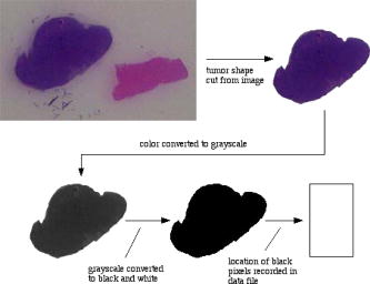
The numerical score is computed to represent four important variants affecting tumor size and reflecting rate of growth. Tumor size is calculated by direct measurement. Pleomorphism is subjectively scored to indicate the degree of variation between individual tumor cells, and reflects both the rate of growth and propensity of tumor cells to organize structures. The shape score represents the irregularity of tumor shape. This shape score is not the same as the shape factor . More aggressive and infiltrative tumors are more irregular, sending projections into surrounding tissue; this, too, indicates pattern of growth (like pleomorphism). Finally, necrosis is based on observation of dead tissue within the tumor, generally related to tumor cells outgrowing their blood supply. Thus, numerical score is taken as a measure of biological (predictive) behavior of the tumor and is typically used by pathologists reviewing surgical biopsies of tumors. The images were proportionally scaled in size from their original size of ( pixels) to a standard size of ( pixels) using Adobe Photoshop 7.0. The images were further processed using Photoshop, as shown in Fig. 1 . As can be seen, the tumor shape was first outlined and cut from the original image in color, then converted to grayscale and then black and white. Figure 2 shows the set of tumor shapes generated after image preprocessing had taken place. The digital resolution of the actual tumor size was . A computer algorithm developed at the Virginia Tech Applied Biosciences Center (VTabc) (Blacksburg, Virginia) was then used to determine the locations of all the black pixels defining the shape and record them in a data file for further processing. All computer algorithms used for analysis of images developed at VTabc were written in the FutureBasic 7.0 computer language and run on a Macintosh G5 computer. In analyzing the images of tumor shapes, we are in fact analyzing a representation of the tumor shape made up of filled-in black pixels. It is clear, in analogy with differential calculus, that the smaller the pixel size and the greater the total number of pixels, the more accurate the representation will become in terms of the area of the representation equaling the actual cross sectional area. In practical terms, however, decreasing pixel size below some given size provides no practical gain. The camera optics, in the final analysis, define the minimum effective pixel size. Having a pixel resolution greater than the associated resolution of the optics serves no purpose. Estimating the perimeter length from those black pixels not entirely surrounded by other black pixels is not quite so straightforward. One cannot simply sum these pixels and obtain a correct result unless the analyzed shape involved is rectangular. Our approach was to weight the contribution to perimeter length by each principal black pixel on the shape surface according to the positions of the black pixels adjacent to it on the surface. A line drawn through the centers of these adjacent surface pixels was used to define the angle of the contribution of the primary pixel to the perimeter. In our case, the contribution could be 1, 1.12, or 1.41. To calculate the shape factor, a computer algorithm was developed to analyze the datasets obtained from the images. The area of the shape was equated with the total number of black pixels in an image, while the length of the perimeter of the shape was equated with the summed edge feature length contributions of all black pixels having at least one white pixel adjacent to them. These feature lengths corresponded to flat surfaces (length contribution=1), surfaces angled at (length contribution=1.12), and surfaces angled at (length contribution=1.41). The angle of the perimeter across the pixel is estimated from the line through the centers of the black pixels along the surface to the left and the right of the pixel being considered. The features utilized, along with their associated weights, are shown in Fig. 3 . Although only one set of features is shown, the analysis included all features equivalent to the ones shown subjected to rotations of multiples of . Once the values of the area and perimeter length were obtained, the shape factor was calculated using Eq. 6. Specifically, after an image was preprocessed to yield a spatial data field of either white (0) or black (1) pixels, the following algorithm was applied to the data field.
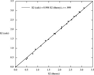
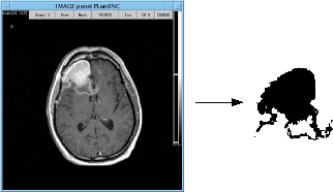
The algorithm was validated using a number of known images whose values of could be calculated theoretically, i.e., filled-in black rectangles with and filled-in black ellipses with (major, minor axes)= , with taking all integer values between 1 and 10. The area of each rectangle= with . The area of each ellipse= , with perimeter estimated using Ramanujan’s approximation,11 i.e., When the theoretically calculated values were compared with the calculated values from the algorithm for the same shapes, very good agreement was found. This is shown in Fig. 4 and allowed us to use the algorithm with some confidence. 4.ResultsData presented in Table 1 show the results of disease-time calculation for rats with implantable hepatomas. A numerical score for each tumor was calculated as a combination of tumor size, tumor shape factor, and two histopathologic variables (cell pleomorphism/variation and necrosis). Using this disease-time score, tumors were classified as being either early, midlife, or late in terms of development and progression. Such a classification would not have been possible if only microscopic morphology was evaluated and is clearly unrelated to absolute tumor size. Some of the tumor sections ended up being quite complex in cross section (tumors 26 and 28), and one tumor displayed an inner void (tumor 35). When the image perimeters were calculated, the entire surface area was included, even the surface area of the void in tumor 35. This was done to minimize the effects of human judgment on the process. We believe that the images as displayed are in fact truly representative of the tumors involved. A plot of shape factor versus disease time is shown in Fig. 5 . As can be seen, the initial shapes have a difference from a circular shape with corresponding high values of . As the small tumors grow and become more regular, i.e., more circular in cross section, decreases and passes through a minimum. At the point at which the tumors become infiltrative, their shapes undergo a structural phase transition and become highly irregular. This is manifested as a large sudden increase in . Finally, as the tumor evolves toward the more regular state at which it would cause a fatality, decreases. 5.DiscussionThese data support the concept that there is significant individual variation in the progression of disease (disease time), and that shape factor analysis may provide an additional important tool for assessing tumor status. In this study, genetically identical rats of the same sex, age, and housed in identical laboratory conditions were transplanted with a well-established neoplastic cell line. As nearly as possible, each animal was treated identically, and yet there was considerable variation at each chronological time point in tumor size, shape, and microscopic morphologic characteristics. Notable were the variations from round and ovoid shapes to more irregular shapes, characterizing later stages of tumor growth, amounts of necrosis in individual tumors, and changes in the organization of tumor cell clusters with advancing disease time. Some features evaluated (amount of inflammatory cell response to the presence of tumor cells) were not considered to be significant. In both clinical practice and in laboratory models of neoplastic growth, an early expansile phase is common. In those neoplasms with more aggressive behavior, the extension of cellular projections from the main tumor mass, sometimes accompanied by penetration of the fibrous capsule around the tumor, is considered to be an indication that some tumor cells are expressing a capacity for motility that may later result in tumor metastasis. In the current model, there are clear transitions in shape factor, and these are correlated with the development of more robust and viable cell clusters late in the course of disease that may be the players in infiltration. Although not examined here, we believe there may be subtle changes in vascularization over the lifespan of the tumor, with midlife tumors outgrowing vascular supply. This may be important, since it may provide both a stimulus for infiltration (i.e., vascular seeking) and for the evolution of new vascular beds later in the lifespan of the tumor that facilitate tumor progression. Work in our laboratory to include a vascular scoring component to the disease-time score is underway. Our work here suggests the need for additional studies to test the entire disease-time paradigm and to see if shape factor analysis is, indeed, correlated highly with tumor progression. We are currently studying shape factors in outcomes of human brain tumors, where infiltrative patterns of growth are common and where patchy necrosis is indicative of irregular growth and vascularization. It is interesting to compare the range of shape values found in this study to those of more complex human cancers such as glioblastoma multiforme. An MRI scan of such a tumor is shown in Fig. 6 along with its preprocessed image. The calculated shape factor for this tumor was , significantly greater than the maximum value of seen in our study of hepatoma. This suggests that this formulation of shape factor might have some utility if applied to other types of cancer. MRI technology, however, allows us to measure shapes in three dimensions in a nonintrusive manner. To make maximum use of this capability, a 3-D shape factor should be used. We define the ratio where is the volume occupied by the shape and is its surface area. The ratio for a sphere is given byIn analogy to our definition of a 2-D shape factor, we define a shape factor for three dimensions,In future MRI-based studies of shape factor versus disease time, we will consider 3-D shapes and use the shape factor defined by Eq. 10.6.ConclusionsThese results demonstrate that tumor growth in groups of genetically identical animals can be quite variable and stress the need to define a bioinformatics dataset (disease time) on which therapeutic decisions could be based. An analysis of tumor shape factor appears to indicate this is an important predictor of progression that should be studied and included as a measure of disease time. It is clear from the great proliferation of shape descriptors that continues to this day that none of them are perfect, even though in general they seek to be invariant to translation, rotation, and scale.1, 12, 13 Perhaps the most simple shape factor, compactness, or area divided by perimeter squared, which is at the heart of our modified shape factor definition, has demonstrated the most usefulness over time. Since compactness is a measure applied to 2-D representations, it does not provide useful information when analyzing multiple shapes when they are part of a single image, or the image is extremely complex and simple coding schemes are employed. Compactness, along with other 2-D shape measures, has a usefulness completely dependent on the relationship between the 2-D image and the 3-D object that it seeks to represent. If this relationship is not consistent and meaningful, then the shape factor analysis will not be meaningful either. We believe that the preliminary research presented in this work suggests that the modified shape factor proposed holds some promise as a method for aiding the determination of disease state and accurate diagnoses. The real promise of this kind of analysis will come, however, when it is combined with the 3-D images that are becoming increasingly available with the more general use of high resolution imaging techniques. ReferencesJ. P. Salmo,
L. Wendling, and
S. Tabbone,
“Automatical definition of measures from the combination of shape descriptors,”
986
–990
(2005). Google Scholar
R. M. Rangayyan,
N. R. Mudigonda, and
J. E. Desautels,
“Boundary modelling and shape analysis methods for classification of mammographic masses,”
Med. Biol. Eng. Comput., 38 487
–496
(2000). https://doi.org/10.1007/BF02345742 0140-0118 Google Scholar
Image-Processing Techniques for Tumor Detection, Marcel Dekker, New York (2002). Google Scholar
R. M. Rangayyan,
N. M. El-Faramawy,
J. E. Desautels, and
O. A. Alim,
“Measures of acutance and shape for classification of breast tumors,”
IEEE Trans. Med. Imaging, 16 799
–810
(1997). https://doi.org/10.1109/42.650876 0278-0062 Google Scholar
J. D. Mabrey,
A. Afsar-Keshmiri,
G. A. Engh,
C. J. Sychterz,
M. A. Wirth,
C. A. Rockwood, and
C. M. Agrawal,
“Standardized analysis of UHMWPE wear particles from failed total joint arthroplasties,”
J. Biomed. Mater. Res., 63 475
–483
(2002). https://doi.org/10.1002/jbm.10302 0021-9304 Google Scholar
L. Keyes and
A. C. Winstanly,
“Fourier descriptors as a general classification tool for topographic shapes,”
193
–203
(1999). Google Scholar
B. Wu,
H. Chen, and
W. Liao,
“Matching of brain sections based on fourier descriptors,”
J. Biomed. Eng., 17
(4), 437
–439
(2000). 0141-5425 Google Scholar
Y. Zheng,
M. S. Nixon, and
R. Allen,
“Lumbar spine visualisation based on kinematic analysis from videofluoroscopic imaging,”
Med. Eng. Phys., 25
(3), 171
–179
(2003). https://doi.org/10.1016/S1350-4533(02)00182-0 1350-4533 Google Scholar
W. B. Spillman Jr., J. L. Robertson,
W. R. Huckle,
B. S. Govindan, and
K. E. Meissner,
“Complexity, fractals, disease time and cancer,”
Phys. Rev. E, 70 061911
(2004). https://doi.org/10.1103/PhysRevE.70.061911 1063-651X Google Scholar
R. Osserman, Survey of Minimal Surfaces, Dover Publications, New York (2002). Google Scholar
B. Berndt, Ramanujan’s Notebooks, Springer Verlag, New York (1985). Google Scholar
T. Bernier and
J. A. Landry,
“A new method for representing and matching shapes of natural objects,”
Pattern Recogn., 36
(8), 1711
–1723
(2003). https://doi.org/10.1016/S0031-3203(02)00352-7 0031-3203 Google Scholar
D. Zhang and
G. Lu,
“Review of shape representation and description techniques,”
Pattern Recogn., 37
(1), 1
–19
(2004). https://doi.org/10.1016/j.patcog.2003.07.008 0031-3203 Google Scholar
|