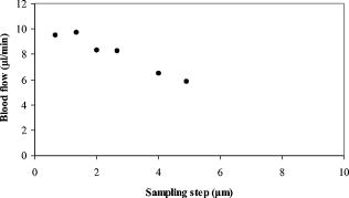
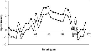
1.

Introduction

Optical coherence tomography (OCT)¹ provides high-resolution cross-sectional imaging^{2, 3, 4, 5, 6} and is commonly used in the diagnosis and management of retinal diseases^{7, 8, 9} and glaucoma.^{10, 11} In addition to obtaining morphological images, OCT can also detect a Doppler shift of reflected light, which provides information about flow and movement.^{12, 13, 14} Several investigators have studied the visualization of blood flow and flow dynamics using Doppler OCT,^{15, 16, 17, 18, 19} but the measurement of the total flow velocity and volume requires additional information about the incident angle between the OCT probe beam and the blood vessel. This information is not available within a single cross-sectional OCT image. Determination of the incident angle requires three-dimensional (3-D) imaging of the blood vessel using more than one cross-sectional scan. Measurement of flow in branch retinal vessels in vivo has recently been accomplished using Doppler Fourier domain OCT (FD-OCT).^{20, 21} Phantom flow measurements showed²² that the difference between the measured flow and actual flow is less than 10%. However, sequentially imaging each retinal blood vessel is time-consuming and not a practical way of measuring the total retinal perfusion in a clinical setting. It is desirable to measure the total retinal blood flow in a single scan. Three-dimensional circular scan imaging has been proposed as a method for measuring retinal blood flow.²³ However, 3-D imaging of the peripapillary area requires many seconds and cardiac cycles, and the measurement of several flow values within a cardiac cycle was demonstrated for an arc scan across only two vessels.²³

We describe here a new method of measuring the total retinal blood flow several times within a cardiac cycle using a novel double circular scanning pattern (DCSP). With a Doppler FD-OCT system, we were able to scan all of the retinal blood vessels that branch from the optic nerve head four times per second. An estimate of the total retinal blood flow was averaged over a $2\text{-}\mathrm{s}$ OCT scan. This new technique may allow routine measurement of total retinal blood flow in a clinical setting. This information will be useful in the diagnosis and management of optic nerve and retinal diseases that are associated with poor blood flow, such as glaucoma and diabetic retinopathy.

2.

Theory

In Doppler OCT, light reflected by moving blood incurs a Doppler frequency shift $\left(\Delta f\right)$ proportional to the flow velocity component parallel to the axis of the probe beam. Given the angle direction, the Doppler shift is simplified to

The OCT sampling beam scans a circular pattern on the retina [Fig. 1a ]. In so doing, the probe beam moves on a cone during scanning. The apex of the cone is in the conjugate plane of the transverse scanning mirrors of the OCT system, which is near the nodal point in the eye. The OCT image shows the retinal structure crossed by the scanning cone [Fig. 1b]. The lateral axis is the angular distribution $\theta$ from $0\mathrm{deg}\text{to}360\mathrm{deg}$ , while the vertical axis $D$ shows the depth information from the scanning cone. The zero frequency position, which is equivalent to the path equal in length between sample and reference arm, is defined as $D=0$ . In a 3-D diagram of the circular scanning pattern (Fig. 2 ), the retina is scanned circularly by the probe beam at radii $r_1$ and $r_2$ . A small radius difference $\Delta r_0=r_2-r_1$ is chosen so that the course of the blood vessel segment VE between the scanning circles is approximately a straight line. In the coordinates shown in Fig. 2, the two positions of the blood vessel segment VE on the two scanning cones have coordinates $P_1(r_1,{\theta }_1,z_1)$ , and $P_2(r_2,{\theta }_2,z_2)$ , respectively. The vector of the blood vessel can be expressed as ${\mathbf{r}}_{\mathbf{b}}$ ( $\Delta x=r_1\cos {\theta }_1-r_2\cos {\theta }_2$ , $\Delta y=r_1\sin {\theta }_1-r_2\sin {\theta }_2$ , $\Delta z=z_1-z_2$ ). In OCT images, the retinal structure matches a coordinate system defined by [ $\theta$ , $D$ in Fig. 1b]. The blood vessel segment VE has relative positions ( ${\theta }_1$ , $D_1$ ) and ( ${\theta }_2$ , $D_2$ ) in the two OCT images with different radii. Thus, the relationship between $\Delta D=D_1-D_2$ and $\Delta z$ can be deduced as

Fig. 1

Circular scan pattern of FD-OCT sampling beam. (a) The circular retinal OCT scan beam rotates in a cone pattern. The apex of the cone is the nodal point of the eye. (b) The cylindrical OCT image is unfolded to fit a rectangular display where the horizontal axis corresponds to the scanning angle from $0\text{to}360\mathrm{deg}$ . The vertical axis corresponds to the depth dimension along the axis of beam propagation.

Fig. 2

Three-dimensional diagram of the OCT beam scanning in a circular pattern across the retina. Two scanning radii, $r_1$ and $r_2$ , are shown in this diagram. See text for symbols.

During scanning, the probe beam BN (Fig. 2) is on the scanning cone. The nodal point $N$ has a coordinate of $(0,0,h+z_0)$ , where $z_0$ is the distance between the retina and the xy plane (Fig. 2). For OCT scans at radius $r$ , when the probe beam scans to the angle $\theta$ , the scanning point B on the retina has the coordinate ( $r\cos \theta$ , $r\sin \theta$ , $z_0$ ). Thus, the vector of the scanning beam BN is $\mathbf{s}$ ( $r\cos \theta$ , $r\sin \theta$ , $-h$ ). With vector $\mathbf{s}$ and ${\mathbf{r}}_{\mathbf{b}}$ , the angle $\alpha$ between the OCT probe beam and blood flow can be calculated as

Assuming that, the relative flow profile does not change during the short sampling period of $2\mathrm{s}$ , the volumetric flow $F$ can be calculated as

Fig. 3

The angle $\beta$ between the OCT plane $S_o$ and the plane normal to the flow direction $P_v$ is indicated. Generation of a Doppler signal depends upon the FD-OCT plane $S_o$ , which crosses the blood vessel, being different from plane $P_v$ , which is normal to the direction of blood flow.

To determine the actual volumetric flow in the blood vessel, the integration should be done in the plane $P_v$ that is normal to the blood vessel (flow) direction. But in practice, the sampled Doppler FD-OCT plane $S_0$ (Fig. 3) that crosses the blood vessel is different from plane $P_V$ in most cases, or there would be no Doppler signal. The relationship between area size ${\sigma }_s=r\Delta \theta \Delta D$ in the OCT plane $S_0$ and area size ${\sigma }_v=\Delta x_v\Delta z_v$ in the plane $P_V$ is ${\sigma }_v={\sigma }_s\mid \cos \beta \mid$ , where $\beta$ is the angle between planes $P_V$ and $S_0$ . According to geometrics, the angle between two planes can be calculated by two vectors that are normal to them separately. For $P_v$ , the vector that is perpendicular to it is the flow vector ${\mathbf{r}}_{\mathbf{b}}$ . The FD-OCT plane $S_0$ is on the scanning cone (Fig. 3). The unit vector ${\mathbf{r}}_{\mathbf{s}}$ , which is perpendicular to plane $S_0$ , is in the plane determined by the probe beam NB and the rotation axis NO, and perpendicular to NB. The unit vector ${\mathbf{r}}_{\mathbf{s}}$ can be deduced as $(\cos \delta \cos \theta ,\cos \delta \sin \theta ,\sin \delta )$ , where $\delta$ is the angle between NB and NO (Fig. 3). With ${\mathit{r}}_{\mathit{b}}$ and ${\mathit{r}}_{\mathit{s}}$ , the angle $\beta$ can be calculated. Thus, the retinal blood flow $F$ can be calculated within the vessel region $S$ in the sampled Doppler FD-OCT image as

3.

Experiment Methods

3.2.

Image Sampling and Processing

The FD-OCT system was coupled to a retinal scanning setup mounted on a slit-lamp biomicroscope. The chin and forehead of the subject rested on a frame in front of the objective lens. A green flashing cross target was used to fix the subject’s gaze. The FD-OCT probe beam was scanned in circular patterns on the retina around the optic nerve head at radii $r_1$ and $r_2$ (Fig. 4 ) using a pair of high-precision optical scanners (6810P, Cambridge Technology, Inc., Cambridge, Massachusetts). Sinusoidal voltage drive signals were generated by InVivoVue imaging software (Bioptigen, Inc., Research Triangle Park, North Carolina) and were triggered to start the scan at the beginning of an FD-OCT frame acquisition. As circular scans are used, the duty cycle of the drive signals is 99.3%, with the scanners returning to their original position at the end of one scan. Shifts between radii were conducted automatically between scans. The scanning radii of 1.8 and $2.0\mathrm{mm}$ were chosen so that the probe beam incidence angle onto the retinal vessels was slightly off-perpendicular, making the Doppler signal for all the retinal branch veins within the the detection range. There were 3000 A-lines sampled in each circle. The phase differences for every three A-lines were calculated to get the Doppler frequency shift. Thus, each frame consisted of 1000 vertical lines. Data was acquired, processed, and streamed to disk for real-time display of Doppler FD-OCT at 4.2 frames per second ( $\mathrm{VC}++$ software, Bioptigen). There were four pairs of Doppler FD-OCT images sampled for each flow measurement. Four were sampled at radius $r_1$ , and four were from radius $r_2$ . The total recording time for the eight-image set was approximately $2\mathrm{s}$ . The sampled Doppler FD-OCT images were saved for further off-line data processing.

Fig. 4

Path of the scanning beam in the double circular scanning pattern. For vessel ${\mathrm{V}}_{\mathrm{S}}$ , the scanning length was $1\mathrm{mm}$ .

Blood flow in the vessels was calculated in a semiautomatic fashion. The locations of the vessels were selected by a human operator (coauthor Y.W.) and then the flows were automatically calculated according to Eqs. 1, 2, 3, 4, 5. The distance $h$ from the nodal point N to the retina surface was assumed to be $17\mathrm{mm}$ according to a standard eye model.²⁵ The speed profile of a single vessel in the eight Doppler images was calculated. Peak velocity in the eight flow profiles was normalized to the maximum one and plotted against time to show the flow pulsation. This curve was integrated as the pulsation term $k$ in Eq. 5. The maximum flow speed profile of the eight analyzed flow profiles was used in Eq. 5 as $A_p$ to calculate the retinal blood flow $\left(F\right)$ . For some veins, the Doppler flow signal was too weak for accurate reading at diastole, the minimum flow portion of the cardiac cycle. For those occasions, the pulsation factor $k$ in the adjacent veins was used for flow calculation.

4.

Results

The in vivo retinal flow measurement was performed on the right eye, and the Doppler FD-OCT images were recorded using the circular scanning protocol. Flow within the major branch retinal blood vessels around the optic nerve head was visible in these images (Fig. 5 ). We chose to measure flow in the branch veins rather than arteries because the arteries have higher flow velocities that can cause excessive phase wrapping and signal fading. The identification of branch veins among the other vessels distributed around the optic nerve head was based on the recorded Doppler frequency shift and the calculated angle between the probe beam and blood vessel. According to Eq. 1, flow occurring in different directions in the same blood vessel introduces different frequency shifts in the backscattered beam. Knowing the direction of flow helps separate the veins from the arteries that are distributed around the optic disk because blood flow in arteries is away from the nerve head and flow in veins is toward the nerve head.

Fig. 5

Doppler OCT images with grayscale display of the Doppler frequency shift. The horizontal axis shows the scanning angle from $0\text{to}360\mathrm{deg}$ . (a) Circular scan at a radius of $1.8\mathrm{mm}$ ; (b) circular scan at $2.0\text{-}\mathrm{mm}$ radius. Retinal branch veins are labeled from ${\mathrm{V}}_1$ to ${\mathrm{V}}_7$ . The inset window shows vessel ${\mathrm{V}}_4$ as an example of background signal removal.

4.2.

Influence of Sampling Density on Doppler Shift Measurement

In Doppler OCT, the phase difference between sequential axial scans is calculated to determine Doppler frequency shift. Ideally, the phase difference should be compared at the same location. However, for retinal OCT systems, the probe beam scans continuously across the retina and there is a small displacement between sequential axial scans. If the sampling locations were not negligibly small relative to the beam diameter, phase decorrelation would decrease the measured Doppler shift.¹⁸ To evaluate the influence of the sampling step on flow measurement, we measured the volume flow in vivo at different sampling steps with the dual scanning plane method.²⁰ For example the scanning length for vessel ${\mathrm{V}}_S$ in Fig. 4 was $1\mathrm{mm}$ . Flow at each sampling step was measured three times and averaged. For each measurement, the integration time of the camera did not change. The results showed that the measured flow decreased with increased sampling steps (Fig. 6 ). This decrease was notable starting at the sampling step around $1.4\mu \mathrm{m}$ . Therefore, to avoid the influence of phase decorrelation between adjacent axial scans, the sampling step should be shorter than $1.4\mu \mathrm{m}$ . In our Doppler FD-OCT system, we chose a 3000 axial line sampling density for real-time display at $4.2\mathrm{Hz}$ . At a scanning radius of $1.9\mathrm{mm}$ (circumference $11.93\mathrm{mm}$ ), the sampling step was about $4.0\mu \mathrm{m}$ . The ratio between the measured flow at the $4.0\text{-}\mu \mathrm{m}$ and $0.7\text{-}\mu \mathrm{m}$ step was 0.683 (Fig. 6). Because the phase decorrelation between adjacent axial lines is mainly related to the beam spot size on the retina,¹⁸ which is a system factor, we used the curve in Fig. 6 to correct the measured flow result for a fixed sampling step.

Fig. 6

Influence of sampling step on the measured volume of blood flow. For sampling steps greater that $1.4\mu \mathrm{m}$ , the estimate of blood flow decreased.

4.3.

Removal of Background Doppler Signal Due to Eye Motion

The Doppler information contained artifacts from the motion of the eye and the OCT system. Doppler noise due to these movements was larger than the phase instability of the OCT system and would have influenced the measurement result if uncorrected. In the Doppler shift image, retinal motion varied across the transverse dimension [Figs. 5a and 5b]. Therefore, the background axial motion of the retina relative to the OCT system was measured locally and used to correct the measured blood flow in the local area.

As an example of how the motion artifacts and OCT limitations were mitigated, consider vessel ${\mathrm{V}}_4$ in Fig. 5 (b, inset). For each axial line, the Doppler signal between the inner retina boundary and vessel boundary was averaged. This value was the Doppler signal due to local tissue motion and was subtracted from the Doppler signal in the whole axial line to get the net signal induced by blood flow. One axial line Doppler signal, noted as the dashed line in Fig. 5 (b, inset), was determined before and after background motion removal (Fig. 7 ). The averaged tissue motion speed was $-0.89\mathrm{mm}∕\mathrm{s}$ . Through subtracting the background motion signal, the averaged Doppler signal was $0.081\mathrm{mm}∕\mathrm{s}$ outside the vessel. After subtraction, the integration of flow was done over the area that contained the vessel. It was not necessary to determine the exact vessel boundary because the net Doppler signal outside blood vessels was close to zero.

Fig. 7

Correction of the Doppler noise due to background motion. The solid curve shows the original signal. The dashed curve shows the Doppler signal after background removal.

4.4.

Volume Blood Flow Results

The first vessel, ${\mathrm{V}}_1$ in Figure 5b, had a negative frequency shift with positive phase wrapping at the center. After phase unwrapping, the flow profile $A(\theta ,D)$ was obtained. The vector of the vessel ${\mathrm{V}}_1$ was calculated as ${\mathbf{P}}_{\mathbf{1}}{\mathbf{P}}_{\mathbf{2}}$ $(-154,-128,-71.34)$ based on the vessel positions in two adjacent images. From Eq. 3, the angle between the scanning beam and blood vessel was calculated as $\cos \alpha =0.24$ , and $\alpha =76.1\mathrm{deg}$ . Since the signal had a negative frequency shift and $\cos \alpha >0$ , the direction of the flow in ${\mathrm{V}}_1$ was from $P_2$ to $P_1$ . In our scanning pattern, $P_1$ was on the inner cone closer to the nerve head, while $P_2$ was on the outer cone. Thus, this flow was toward the optic disk; therefore, blood vessel ${\mathrm{V}}_1$ was a vein. Through continuous scanning, eight frames of the Doppler signals were recorded. The flow speed at the center part of vessel ${\mathrm{V}}_1$ [Fig. 5b] was analyzed, and the normalized flow speed was plotted (Fig. 8 ). The cardiac pulsation factor, calculated based on the curve in Fig. 8, was $k=0.695$ . With the value of $\cos \alpha$ , the calculated peak flow speed in ${\mathrm{V}}_1$ was $17.0\mathrm{mm}∕\mathrm{s}$ . From Eq. 5, the angle $\beta$ was calculated as $\cos \beta =-0.97$ . With these parameters, the volumetric flow in vessel ${\mathrm{V}}_1$ was calculated as 3.01 $\mu \mathrm{l}∕\min$ . Considering the effect of phase decorrelation due to insufficient sampling density (Fig. 6), the adjusted volumetric flow was $4.41\mu \mathrm{l}∕\min$ .

Fig. 8

Normalized peak flow speed variation with time for the vessel ${\mathrm{V}}_1$ shown in Fig. 6.

The flow directions of the main vessels around the optic nerve head were similarly analyzed, and the main venules were identified and labeled ${\mathrm{V}}_1\text{to}{\mathrm{V}}_7$ [Fig. 5b]. The blood flow for each venule was calculated (Table 1 ). The summation of these flows determined the total venous flow out of the retina, which was $53.87\mathrm{\mu l}∕\min$ . The scanning angle between the probe beam and blood vessel was also determined (Table 1).

Table 1

Vessel diameter, scanning angle, and flow volume for the retinal branch veins of the first subject.

	Vessel
	V1	V2	V3	V4	V5	V6	V7
Diameter $\left(\mu \mathrm{m}\right)$	70.3	78	152	70	126	115	96
Angle (deg)	76.1	78.8	85.9	96.6	94.25	84.4	81.3
Volume flow $(\mu \mathrm{l}∕\min )$	4.41	2.88	13.89	3.50	9.94	11.58	7.67

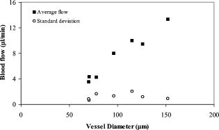
There were seven measurements performed upon this subject in which the total venous flow was calculated for each measurement. The total sampling time was finished within $10\min$ . The averaged total flow was $52.90\mathrm{\mu l}∕\min$ , with a standard deviation of $2.75\mathrm{\mu l}∕\min$ , which is about 5.2% of the average flow. Collectively, vessels with larger diameters had higher flow rates than did smaller vessels (Fig. 9 ). The flow rates ranged from $3.53\mathrm{\mu l}∕\min$ in the smallest vessel to $13.32\mathrm{\mu l}∕\min$ in the largest vessel, with standard deviations ranging from $0.69\text{to}2.08\mathrm{\mu l}∕\min$ .

Fig. 9

Relationship between vessel diameter and volume blood flow.

To test the reliability of this method, flow rates were measured in another subject. The left eye of the subject was scanned six times. Each scan was finished within $2\mathrm{s}$ , within which eight Doppler FD-OCT frames were acquired. The total measuring time was finished within $10\min$ . Through similar data analysis, we found a total of 5 main branch veins identified from the Doppler image. Based upon the six sets of sampled data (Fig. 10 ), the average flow was $45.22\mathrm{\mu l}∕\min$ . The standard deviation of the total flow for this subject was $3.18\mathrm{\mu l}∕\min$ , which was 7.0% of the average flow. The average flow for both subjects was $49.07\mathrm{\mu l}∕\min$ , with a difference of $7.67\mathrm{\mu l}∕\min$ between the two subjects.

Fig. 10

Repeatibility measurement for the second subject.

5.

Discussion

By using the DCSP method, we demonstrated that the total retinal blood flow can be determined rapidly. The measured total retinal venous flow in one volunteer, $52.90\mathrm{\mu l}∕\min$ , was close to the value of $54.71\mathrm{\mu l}∕\min$ that was previously measured by sequentially imaging each retinal blood vessel individually.²⁰ We targeted the major branches of the central retinal veins because the sizes and velocities were within the dynamic range of the Doppler FD-OCT system. Because the total venous flow volume is identical to that of arteries in the retina, as shown by Riva and colleagues,²⁶ measuring the total venous flow alone is sufficient to quantify the total retinal blood flow. With the laser Doppler flowmeter (LDF) technique, the early study reported total venous flow of $34.0\pm 6.3\mu \mathrm{l}$ /min from normal human subjects.²⁶ In another study using LDF,²⁷ the total venous flow was $64.9\pm 12.8\mathrm{\mu l}∕\min$ in the normal human eye. The measured average total venous flow in our study, 52.90 and $45.23\mathrm{\mu l}∕\min$ for the two normal subjects, was within the range of these previously published values.

There are some limitations to our technique. The assumed distance between the nodal point of the eye and the retinal plane may vary due to eye length variation and, to smaller extents, the refractive error and instrument positioning variation. However, our calculations show that nodal point position has very little effect on the measured blood flow. For example, the normal human eye has a length that ranges between $21\text{to}26\mathrm{mm}$ . The distance $h$ from the nodal point to the retina is about 70% of eye length. So $h$ is between 14.7 and $18.2\mathrm{mm}$ , a difference of $3.5\mathrm{mm}$ . The flow measurement error in a very short $\left(21\mathrm{mm}\right)$ or long $\left(26\mathrm{mm}\right)$ eye would be only $\pm 0.7\%$ relative to the average eye $\left(24\mathrm{mm}\right)$ .

A second potential limitation is that our frame rate of $4.2\mathrm{Hz}$ was barely enough to track the variation in flow velocity during the cardiac cycles. We believe that a higher frame rate would improve the accuracy of our measurements. Third, our transverse sampling interval of $4.0\mu m$ , due to a scanning diameter of $1.9\mathrm{mm}$ for 3000 axial sampling lines, was not sufficient to avoid phase decorrelation in the adjacent axial lines. A correction factor based on calibration measurements had to be used to calculate the volume of retinal flow. Four, branch veins with diameters less than $65\mu m$ were not taken into account due to limited lateral sampling density. A finer sampling interval could decrease the phase decorrelation effect and allow flow measurement in smaller vessels, thereby increasing the measurement accuracy. Fifth, in some arteries during systole, the Doppler velocity was unreadable due to fading of the OCT signals. We believe that this is due to the velocity-related interferometric fringe washout. If the reflector moves by more than a quarter wavelength within the spectrometer’s integration time of $50\mu s$ , the peaks and troughs of the interference signal average out. Sixth, at high flow speeds, the Doppler phase shift can exceed $\pi$ , causing “phase wrapping.” A very high flow that causes phase wrapping over one period is too complex for the computer software to analyze reliably. Thus, a shorter integration time could extend the upper limit of measurable velocity. Last, eye movement in the depth dimension affects the accuracy of retinal vessel depth and incidence angle measurements.²³ This is especially critical for blood vessels that are nearly perpendicular to the OCT beam—since the precision of the incidence angle was $1.42\mathrm{deg}$ , the incidence angle on the blood vessel should be at least twice $1.42\mathrm{deg}$ from perpendicular to permit reasonable velocity measurement. We found that in the $3.6\text{to}4.0\mathrm{mm}$ -diam circles around the optic disk, the vessels sloped upward as they emerged from the disk, providing a good range of incidence angle for Doppler blood flow measurement.

Most of the preceding limitations can be reduced with greater imaging speed. Decreasing the effective integration time of the spectrometer can increase the detectable range of flow speeds. A higher speed will also allow for a finer degree of sampling in time, i.e., more time points within each cardiac cycle. It will also allow a finer degree of sampling in space, i.e., more points sampled within each blood vessel. At high sampling speed, incidence angle measurement error due to eye motion will also be reduced. With the continual improvement in the speed of line cameras that make up the heart of the FD-OCT system, we can expect these limitations to become less important over time. Despite all these limitations, we were able to achieve our main goal of measuring total retinal blood flow in the venous system several times within a cardiac cycle.

Several methods of visualizing and measuring retinal blood perfusion already exist.^{28, 29, 30, 31, 32} Fluorescein angiography²⁹ allows visualization of retinal hemodynamics but does not measure volumetric blood flow. The pulsatile ocular blood flowmeter (POBF Paradigm, Inc.)²⁸ measures both uveal and retinal blood flow. The POBF assumes a scleral rigidity that relates intraocular pressure and eye volume. Scleral rigidity is likely to vary significantly between people, introducing a major source of measurement variation. There are two types of LDF on the market: the Canon (Canon U.S.A., Inc., Lake Success, New York,) and the Heidelberg (Heidelberg Engineering, GMBH, Heidelberg, Germany). The Heidelberg retina flowmeter (HRF)³⁰ measures in arbitrary units flow in the retinal capillary bed over a small region. It is suitable for measuring local perfusion variation but cannot measure the total retinal blood flow,³¹ which reflects on the global health of the eye. The Canon flowmeter (CF) is closer to our methods in that it measures flow at points within the large retinal branch vessels. To convert the velocity measurements to flow estimates, it assumes a fixed relationship between the maximum detected Doppler shift and the average velocity within the blood vessel.^{32, 33} To measure the total retinal blood flow, the CF requires careful positioning of the scan on each major retinal branch blood vessel, which is a time consuming process. Thus, none of the current retinal blood flow measurement technologies are able to provide rapid (faster than the cardiac cycle) measurements of total retinal blood flow.

The DCSP method reported in this paper produces an absolute flow measurement by integrating the flow profile of the blood vessel cross section without resorting to any assumptions on the anatomic or flow parameters. Flow pulsation was averaged over cardiac cycles sampled within $2\mathrm{s}$ for volume flow calculation. This will greatly reduce the chair time for the photographer and patient in the clinic.

The measurement of total retinal blood flow is important for the treatment of some eye diseases. The leading causes of blindness in the United States,^{34, 35, 36} such as diabetic retinopathy and age-related macular degeneration, are related to vascular abnormalities. Central retinal vein occlusion and branch retinal vein occlusions are also common retinal diseases characterized by decreased retinal blood flow. Glaucoma is another leading cause of blindness that is primarily linked to elevated intraocular pressure; however, poor circulation in the retina and optic nerve is thought to be a risk factor for glaucoma disease progression as well.^{37, 38} Glaucoma causes atrophy of the inner retinal layers served by the retinal circulation. Therefore, measurement of the total retinal blood flow may also be a useful approach to assess the severity of glaucoma in an eye. A rapid and accurate measurement of total blood flow with Doppler OCT could enhance our understanding of pathophysiology and develop treatments that improve retinal blood flow for these diseases.

6.

Conclusion

In summary, we present in vivo measurements of retinal blood flow using Doppler FD-OCT. A DCSP was developed to determine the angle between the blood flow and scanning beam so that the real flow velocity can be measured. Volumetric flow in the branch veins around the optic nerve head was integrated in the sampled cardiac cycles. The measured blood flow for two subjects was $52.90\pm 2.75$ and $45.23\pm 3.18\mathrm{\mu l}∕\min$ , with a difference of $7.67\mathrm{\mu l}∕\min$ . This method will be useful for the measurement of total retinal blood flow quickly without depending on any assumption of vessel size or flow profiles.