Low-frequency wide-field fluorescence lifetime imaging using a high-power near-infrared light-emitting diode light source

Sylvain Gioux; Stephen J. Lomnes; Hak Soo Choi; John V. Frangioni M.D.

doi:10.1117/1.3368997

1 March 2010 Low-frequency wide-field fluorescence lifetime imaging using a high-power near-infrared light-emitting diode light source

Sylvain Gioux, Stephen J. Lomnes, Hak Soo Choi, John V. Frangioni M.D.

Author Affiliations +

Journal of Biomedical Optics, Vol. 15, Issue 2, 026005 (March 2010). https://doi.org/10.1117/1.3368997

Abstract

Fluorescence lifetime imaging (FLi) could potentially improve exogenous near-infrared (NIR) fluorescence imaging, because it offers the capability of discriminating a signal of interest from background, provides real-time monitoring of a chemical environment, and permits the use of several different fluorescent dyes having the same emission wavelength. We present a high-power, LED-based, NIR light source for the clinical translation of wide-field (larger than 5 cm in diameter) FLi at frequencies up to 35 MHz. Lifetime imaging of indocyanine green (ICG), IRDye 800-CW, and 3,3-diethylthiatricarbocyanine iodide (DTTCI) was performed over a large field of view (10 cm by 7.5 cm) using the LED light source. For comparison, a laser diode light source was employed as a gold standard. Experiments were performed both on the bench by diluting the fluorescent dyes in various chemical environments in Eppendorf tubes, and in vivo by injecting the fluorescent dyes mixed in Matrigel subcutaneously into CD-1 mice. Last, measured fluorescence lifetimes obtained using the LED and the laser diode sources were compared with those obtained using a state-of-the-art time-domain imaging system and with those previously described in the literature. On average, lifetime values obtained using the LED and the laser diode light sources were consistent, exhibiting a mean difference of 3% from the expected values and a coefficient of variation of 12%. Taken together, our study offers an alternative to laser diodes for clinical translation of FLi and explores the use of relatively low frequency modulation for in vivo imaging.

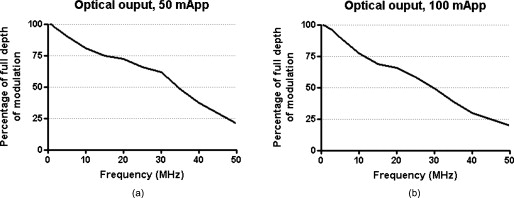
1. Introduction

Over the past decade, wide-field, noncontact optical imaging has made tremendous progress toward solving important clinical problems. Continuous-wave (CW) fluorescence has been successfully translated to clinical trials^{1, 2, 3, 4, 5, 6, 7} and paves the way for many other optical techniques. Modulating the light source in space or time allows for improved fluorescence detection^{8, 9, 10, 11}, and for recovery of endogenous optical properties of tissues (i.e., absorption and scattering coefficients).^{12, 13, 14, 15} Therefore, the translation of a wide-field, modulatable light source in the context of fluorescence imaging is of special interest. For instance, many fluorescence techniques require the intravenous injection of an exogenous fluorophore, which binds to a target, but which also typically clears incompletely from surrounding tissue, leading to a reduced signal-to-background ratio (SBR). Currently, the only solution to this problem is to design fluorescent probes that clear quickly from the body, resulting in a sufficiently high SBR.^{16, 17}

Another possible solution is the imaging of fluorescence lifetime (FLi). There are four main advantages with this technique. First, one can design a fluorescent probe whose lifetime is significantly different from endogenous fluorescence lifetimes.¹⁸ Second, fluorescence lifetime varies between the bound and unbound state.¹⁹ Third, lifetime varies with chemical environment, which permits functional imaging.^{20, 21} And, last, probes with different lifetimes could be used to image several targets using only a single excitation wavelength.

Presently, however, clinical imaging systems that perform fluorescence lifetime imaging are not readily available. One of the major roadblocks to such systems is the design of a light source capable of producing safe, high-power illumination that is modulated at high frequency. Laser diode–based imaging systems, at the power required for wide-field imaging, would require laser goggles and special operating room precautions. LEDs, on the other hand, are particularly attractive for clinical translation because they are safe, inexpensive, efficient, and available at many different wavelengths, and they have relatively narrow illumination bands. There has been some previous work using LEDs for FLi in wide-field microscopy.^{22, 23, 24} but our interest here is focused on macroscopic, surgical-scale wide-field (typically $10 cm$ in diameter) subsurface fluorescence imaging. In this application, optical power requirements are significant.

In this article, we lay the foundation for the clinical translation of fluorescence lifetime imaging. First, we describe an optimization of parameters for performing frequency-domain imaging (FDi) of fluorescence lifetimes in a clinical context. This includes the choice of the modulation frequency and its effect on lifetime recovery. We then introduce an LED-based light source specifically designed to modulate 12 high-power, $5 - mm$ epoxy LEDs simultaneously and in phase. We validate the optical performance of this LED light source and compare it to the gold standard FLi light source, a laser diode, under both bench and in vivo conditions.

2. Optimized Fluorescence Lifetime Imaging (FLi)

2.1.

General Description

Fluorescence lifetime imaging (FLi) has been studied extensively.^{8, 9, 10, 19, 25, 26, 27, 28, 29, 30} Some of the most common applications include fluorescence lifetime determination using ultraviolet (UV) and blue wavelengths.^{31, 32} Recently, there has been significant interest in using NIR wavelengths for exogenous fluorescence lifetime imaging.^{21, 33, 34} Several approaches are possible to perform FLi. The most intuitive is time-domain imaging (TDi), where short pulses (ps to fs) of laser light are delivered to the sample.^{12, 35, 36} The fluorescence signal is then detected using short acquisition gates synchronized with the illumination pulse. Scanning this gate in time permits the recovery of fluorescence lifetime. Another approach is to use frequency-domain imaging (FDi).^{8, 25, 37} In this case, one uses an intensity-modulated illumination at a frequency from several tens to hundreds of MHz. Relative to excitation, the emitted fluorescence intensity will be shifted in phase due to its lifetime decay. Instead of delaying a gate in time for detecting the fluorescence decay, an image intensifier, modulated in gain, is shifted in phase relative to the excitation light, and the fluorescence signal’s phase is measured. The image intensifier gain modulation frequency can be the same as the illumination and phase-shifted to perform homodyne detection, or slightly different to perform heterodyne detection.

The main performance difference between TDi and FDi resides in practical implementation, since they are theoretically the exact Fourier transform of one another. Sources used in TDi are often expensive, resulting in an overall cost higher than FDi. Imaging of wide fields of view (FOVs) in TDi can be challenging, whereas in FDi, it can be performed easily by taking advantage of the multipixel detectors of conventional CCD cameras.^{8, 37} For these reasons, we chose to implement a frequency-domain approach to explore the potential for clinical translation of FLi.

2.2.

Optimizing in vivo Lifetime Detection in FDi

A major issue with in vivo measurements of lifetime in living tissues is photon propagation delays due to scattering. When tissue optical properties are well known, these delays can be predicted and fluorescence lifetime estimated.^{13, 38, 39} However, optical properties are not always known. In this case, one can use a fluorescence lifetime reference probe inside the tissue to minimize the influence of scatterers and recover lifetime of the unknown probe.⁹ The main assumption is that the optical properties contribute similarly to both the region under interrogation and to the reference lifetime and therefore can be accounted for.

In the absence of scatterers, the relationship between phase and lifetime for mono-exponential decay can be expressed using Eq. 1:

Eq. 1

τ = \frac{\tan (θ)}{2 π f},

where

τ

is the unknown lifetime,

θ

is the phase referenced to the illumination, and

f

is the frequency of illumination. Equation 1 highlights the nonlinear nature of the relationship between phase and lifetime at a single frequency

f

. It is therefore nonintuitive to understand the relationship between phase and lifetime. Of particular interest is the choice of the frequency of illumination, which is directly linked to an important parameter, the minimum phase detectable by the imaging system. The latter is mainly determined by the phase resolution of the signal generators and the noise of the image intensifier.

The phase difference $Δ θ$ between two probes with known lifetimes $τ_{1}$ and $τ_{2}$ is expressed as:

Eq. 2

Δ θ = θ_{2} - θ_{1} = \arctan (2 π f τ_{2}) - \arctan (2 π f τ_{1}) .

To understand the relationship between phase difference and modulation frequency [Eq. 2], we used MATLAB to compute and plot in Fig. 1 the phase difference between an unknown dye and indocyamine green (ICG) in vivo [

0.67 - ns

lifetime; obtained in 100% serum using time-domain measurement³⁶ and verified against literature values from Akers ]³⁴ at various modulation frequencies (20, 40, 60, 80, and

100 MHz

). It is interesting to note that above

60 MHz

, there is little benefit in increasing the modulation frequency when comparing fluorescent dyes with lifetime values similar to that of ICG. In this case, working at relatively low frequency is possible, with few disadvantages.

Fig. 1

Optimization of modulation frequency for frequency-domain imaging (FDi) of fluorescence lifetimes: (a) Phase difference between ICG in vivo $(τ_{1} = 0.67 ns)$ and a fluorescent dye of lifetime $τ_{2}$ at various illumination frequencies according to Eq. 2. (b) Measured lifetime of an unknown fluorophore relative to the phase difference with ICG in vivo at high $(100 MHz)$ and low ( $35 MHz$ ; used this in study) frequencies according to Eq. 3.

When a fluorescent target of unknown lifetime is compared to a reference, the following relationship can be used to recover the unknown lifetime:

Eq. 3

τ = \frac{\tan [\arctan (2 π f τ_{ref}) + (θ - θ_{ref})]}{2 π f},

where

τ

is the unknown lifetime,

τ_{ref}

the reference lifetime,

θ

the phase of the unknown probe,

θ_{ref}

the phase of the reference probe, and

f

the frequency of illumination. In the present study, we chose to modulate the light source at

35 MHz

. Based on Eq. 3, the fluorescence lifetime of ICG (

0.67 ns

;

τ_{ref}

) and the phase resolution limit of our detection system

(5 \deg)

, lifetime differences as short as

0.5 ns

should be resolvable. The comparison curves for measured lifetime versus phase difference at

100 MHz

and

35 MHz

were computed with MATLAB using Eq. 3 and are plotted in Fig. 1. A lower slope for the

100 - MHz

curve indicates better sensitivity to lifetime variation through phase detection; however, the higher slope for the

35 - MHz

curve results in a higher dynamic range. Overall, the data suggest that

35 MHz

should be capable of discriminating

0.5 - ns

differences between ICG and an unknown dye in vivo.

3. Material and Methods

3.1.

LED Light Source

We designed the LED light source to be modular and to accommodate various wavelengths. Each LED module is composed of two elements: an LED printed circuit board (PCB) hosting the LEDs and a driver PCB that supplies power to the LEDs. This permits different LED PCBs to be swapped for use with the same driver PCB. A detailed description of the LED light source is available in Ref. 40 and Gerber files, and parts lists for the PCBs are available at www.frangionilab.org. For clarity, we will introduce briefly the LED PCB and highlight the working principles of the LED driver PCB. Further details are available in Ref. 41.

3.1.1.

LED PCB

$760 - nm$ near-infrared (NIR) $5 - mm - diam$ epoxy LEDs were purchased from Marubeni Epitex (Santa Clara, California; catalog #L760-01AU). These LEDs have a $1.85 - V$ forward voltage, a $10 - \deg$ half angle, and a typical optical power of $18 mW$ when driven at $50 mA$ . A custom PCB hosting the LEDs was fabricated by Nashua Circuits (Nashua, New Hampshire) and assembled by Sure Design (Farmingdale, New Jersey). More details about the LED PCB are available in Ref. 40.

3.1.2.

Driver PCB

A typical LED driver involves a resistor connected in series with the LED, setting an operating point onto the voltage-current curve of the LED. This allows the control of current flow through the LED and, therefore, its optical output. However, in this case, the current flow will be constant with time. The desired LED driver should be able to modulate the optical output of the LED in time at relatively high frequency (typically, tens of MHz for FLi). One approach would be to modulate the LED forward voltage; however, operating multiple LEDs in series would require high-power modulation. To overcome high-power modulation, one could tune a resonant circuit at the frequency of interest, as suggested in Ref. 22. Although efficient, this approach provides only a single modulation frequency, greatly impairing the flexibility and potential use of LEDs in DC mode or at other frequencies. Another disadvantage of the tuned resonance approach is that the LED fabrication process does not guarantee a well-known current–voltage relationship, which can lead to variations in optical output.

Another approach consists of controlling the current flow through the LEDs.⁴² As illustrated in Fig. 2 , one solution consists of using a combination of an operational amplifier (op-amp), a transistor [here, a metal-oxide semiconductor field effect transistor (MOSFET)], and a resistor. Voltage applied to the positive input of the op-amp will be replicated at the resistor through negative feedback. Therefore, the current flow through the resistor will be simply set by Ohm’s law applied to the resistor potential difference, and imposes the same current flow through the LEDs. The forward voltage is supplied to the LEDs to ensure their proper operation at the desired current. The elegance of this approach resides in the fact that the excess in supply voltage $(V_{supply})$ is stored at the transistor drain. More details on the principles of the driver circuit can be found in Ref. 42.

Fig. 2

High-power, high-frequency linear LED driver circuit: (a) Principle of operation. (b) Practical implementation.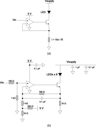

In order to obtain the best possible high-power modulation, attention must be paid to several parameters in the choice of the components. A Maxim (Sunnyvale, California) model no. 4451 operational amplifier was chosen in combination with a Zetex (Diodes Incorporated, Dallas) model no. ZVN3306F MOSFET. The op-amp has been selected for its wide bandwidth ( $210 MHz$ , $- 3 dB$ ) and driving capabilities (rail-to-rail output), and the MOSFET for its low ON resistance $(5 Ω)$ , high drain-source breakdown voltage $(60 V)$ , high current capability $(150 mA)$ , and low input capacitance $(35 pF)$ . Further details about the driver circuitry and its performance are available in Ref. 41.

3.2.

Experimental Setup

Shown in Fig. 3 is the experimental setup used to perform both in vitro and in vivo FLi measurements. Images were collected using a simultaneous color and NIR fluorescence imaging system described in detail previously.⁴³ Briefly, the system consists of NIR-compatible optics collecting light from the region of interest and forming images on two CCD cameras resampled at 640 by $480 pixels$ . A dichroic mirror (model no. HMS3000-Di680, Chroma Technology, Brattleboro, Vermont) split the light into color information $(400 to 650 nm)$ collected by a color camera (model no. Imitech IMC-80F, IMI Technology, Seoul, Korea) and NIR fluorescence emission information $(\approx 800 nm)$ collected by an NIR camera (model no. Orca-AG, Hamamatsu, Bridgewater, New Jersey). A $650 - nm$ shortpass filter (Chroma HMS3000-Em650SP) was used in front of the color camera to prevent blooming artifacts from NIR excitation light. To perform homodyne detection, we added an image intensifier (IIT) model no. FS9910C-268484 (ITT Night Vision, Roanoke, Virginia), in front of the NIR camera. To prevent NIR fluorescence excitation light from reaching the IIT, an $800 -to 848 - nm$ emission filter (Chroma no. HMS3000-Em824/47) was employed (Fig. 3). A custom high-voltage DC power supply for the image intensifier, model no. 2006540-004, was manufactured by GBS Power Supplies (San Jose, California) and was used to set DC voltages for the photocathode (PC), the multichannel plate (MCP), and the screen. The gain of the IIT’s PC was modulated at the exact same frequency as the light source using a high-frequency signal generator model no. IFR2023 (Aeroflex, Plainview, New York) amplified to $\approx 150 Vpp$ using a $25 - W$ high-frequency power amplifier model no. 25A250A (Amplifier Research, Souderton, Pennsylvania). The amplified AC signal was superimposed on the PC DC voltage of the IIT using a custom circuit (GE Global Research, Niskayuna, New York).

Fig. 3

Experimental apparatus. Light reflected from the sample is collected through lenses and separated into color $(400 to 650 nm)$ and NIR fluorescence $(> 800 nm)$ wavelengths using a dichroic mirror and filters. An image intensifier tube (IIT) is modulated at frequency $f$ with a selected phase difference (phase) relative to the light source, permitting homodyne detection.

Two types of light sources were used for our experiments: (1) the LED module described earlier, and (2) a laser diode (considered the gold standard for FLi). For the LED light source, DC input voltage $(V_{in})$ was supplied using a signal generator model no. HP3245a (Hewlett Packard, Palo Alto, California). LED modulation voltage (AC component), from a high-frequency Aeroflex no. IFR2023 signal generator, was superimposed on this $V_{in}$ DC signal using a bias tee model no. ZNBT-60-1W (Mini-Circuit, Brooklyn). Power ( $V_{supply}$ and $5 V$ ) was supplied by a BK Precision (Yorba Linda, California) triple-output power supply model no. 1672. For the laser diode light source, a $100 - mW$ , $785 - nm$ diode model no. L785P100 (Thorlabs, Newton, New Jersey) was mounted in a model no. TCLDM9 (Thorlabs) laser diode mount with thermo-electric cooler (TEC). Laser diode temperature was controlled using a TEC controller model no. TEC200 (Thorlabs). The DC component of the laser diode output was controlled by a model no. LD220C driver (Thorlabs). The AC component was generated using an Aeroflex IFR2023 high-frequency signal generator directly plugged into the TLDCM9 RF input and fed into the laser diode using the internal bias tee. Components were controlled and images were acquired using a custom program written in LabVIEW (National Instruments, Austin, Texas). During FLi experiments, LED and laser light sources were set to identical depths of modulation by means of a $125 - MHz$ photodiode model no. 1801-FS (New Focus, San Jose, California) whose output was visualized using a WaveSurfer oscilloscope model no. 44Xs (LeCroy, Chestnut Ridge, New York). Detector system settings remained unchanged when comparing LED and laser light sources.

3.3.

FLi Experiments

3.3.1.

Bench Experiments

Indocyanine green (ICG) and $3, 3^{'}$ -diethylthiatricarbocyanine iodide (DTTCI) were purchased from Sigma (St. Louis, Missouri), and the carboxylic form of IRDye 800-CW (CW800) was from LI-COR (Lincoln, Nebraska). NIR fluorescent dyes were dissolved in dimethyl sulfoxide (DMSO), 100% serum supplemented with $20 mM$ 4-(2-Hydroxyethyl)piperazine-1-ethanesulfonic acid (HEPES), pH 7.4, or 50% serum in HEPES/50% Matrigel (BD Bioscience, Bedford, Massachusetts), and imaged with the experimental setup. FLi experiments were performed using the homodyne technique, with images acquired alternatively with the LED and the laser diode light sources, at $35 MHz$ , with phase increments of $10 \deg$ , five repetitions per phase value, and over one phase period. ICG in DMSO $(τ_{1} = 0.67 ns)$ was used as our lifetime standard. Lifetime values were compared to those obtained using a well-characterized time-domain imaging system³⁶ and verified against literature values.³⁴

3.3.2.

In Vivo Experiments

Animals were housed in an Association for Assessment and Accreditation of Laboratory Animal Care (AAALAC)–certified facility and were studied under the supervision of an approved institutional protocol. Healthy CD-1 mice of either sex weighing $30 g$ were purchased from Charles River Laboratories (Wilmington, Massachusetts) and anesthetized with $65 mg ∕ kg$ intraperitoneal pentobarbital (Ovation Pharmaceutical, Inc., Deerfield, Illinois).

We used fluorophores $(5 μ M to 10 μ M)$ mixed in Matrigel to prevent the dyes from diffusing into surrounding tissues and the bloodstream after subcutaneous injection. Matrigel is a biocompatible extracellular matrix that is liquid at $4 ° C$ and a rapidly polymerizing gel at body temperature $(37 ° C)$ . Mice were shaved on their dorsal side to expose the skin. The injection locations were marked with black circles on the skin before injection. ICG, CW800, and DTTCI were added to $4 ° C$ Matrigel and injected subcutaneously. FLi experiments were performed using the homodyne technique, with images were acquired alternatively with the LED and the laser diode light sources at $35 MHz$ , with phase increments of $10 \deg$ , five repetitions per phase value, and over one phase period. ICG in Matrigel was used as the lifetime reference, as described for bench experiments.

3.4.

Processing

All images were similarly processed to extract the phase at every pixel location using a custom program written in MATLAB (MathWorks, Natick, Massachusetts). First, the image pixels were binned (5 by 5) to decrease processing time. Each resulting pixel intensity over one phase period was normalized in amplitude, resulting in a 0-to-1 variation in intensity. Last, each pixel over one phase period was fitted to a sine wave and its phase used for fluorescence lifetime estimation. The fit function used was from the Ezfit toolbox, which performs an unconstrained nonlinear minimization of the sum of squared residuals (SSR) with respect to the fitted parameter (here, phase). The motivation for normalizing data from 0 to 1 was justified in improving the fitting time by fitting only for phase and not for amplitude.

Last, the fluorescence lifetime of each binned pixel was extracted using Eq. 3 (see Sec. 2) and the reference fluorophore. Images were displayed using the correlation coefficients from the sine wave fit as a mask. In this way, display is not dependent on fluorescence intensity, but solely on lifetime.

4. Results

4.1.

LED Light Module

Shown in Fig. 2 is the circuit implemented in the driver PCB. It includes decoupling capacitors, loads to stabilize the circuit behavior, and an input bias current compensation. Pictures of the driver PCB are shown in Fig. 4 . Pictures of an LED module containing twelve $5 - mm$ LEDs, pre- and post-molding with thermally conductive silicone, are shown in Fig. 4. More information about the light modules and their use in a clinical fluorescence imaging system is available in Ref. 40. Measured power for one module using a $7 - \deg$ half-angle silicone collimator was $166 mW$ when driving the LEDs at $80 mA$ (Ref. 40).

Fig. 4

LED light module: (a) Back (left) and front (right) of the driver PCB. (b) Mating of the driver PCB and LED PCB by means of two-pins headers, pre- (left) and post-molding (right) with thermally conductive silicone.

4.2.

Module Modulation Performance

Shown in Fig. 5 is the optical output from the LED module shown in Fig. 4 as a function of modulation frequency. Modules were driven at typical operating conditions with $50 - mApp$ current [Fig. 5] or at absolute maximum operating conditions with $100 - mApp$ current [Fig. 5]. Notice that $- 3 - dB$ amplitude modulation is obtained at $35 MHz$ when using the typical operating condition and $30 MHz$ when using absolute maximum operating conditions. More details about the testing procedure and the performances are available in Ref. 41.

Fig. 5

LED light module performance. Optical output of the LED light module (ordinate) versus modulation frequency (abscissa): (a) Typical operating conditions $(50 mApp)$ . (b) Absolute maximum operating conditions $(100 mApp)$ .

4.3.

Bench Experiments

Results from bench fluorescence lifetime measurements are summarized in Table 1 . Values used for the expected lifetimes of ICG, CW800, and DTTCI were obtained from time-domain measurements on a well-characterized instrument³⁶ and verified with literature values from the study of Akers ³⁴ that systematically studied NIR fluorescent dyes lifetime in various chemical environments. Overall, measurements made using our modulated LED module or a conventional laser diode were very similar, and close to the expected lifetimes. Due to the low modulation frequency used $(35 MHz)$ , small variations of phase result in large variations in lifetime [see Fig. 1]. As might be expected, this results in an increased influence of detector noise compared to measurements made at higher modulation frequency. The standard deviation of lifetime measurements was in the range $0.1 to 0.2 ns$ for both the LED module and the laser diode. Instrument noise is discussed in detail below.

Table 1

Summary of bench FLi results. Fluorescence lifetimes of ICG, CW800, and DTTCI in various environments (DMSO, serum, and Matrigel) obtained using LED or laser diode light sources.

	Environment	Fluorescencelifetime using LEDlight source(ns)	Fluorescencelifetime usinglaser diode lightsource (ns)	Expectedfluorescencelifetime (ns)
ICG	DMSO	Used for reference	Used for reference	0.971
	Serum	Used for reference	Used for reference	0.681
	Matrigel	$0.53 \pm 0.09$	$0.55 \pm 0.07$	NA
CW800	DMSO	$1.24 \pm 0.13$	$1.29 \pm 0.12$	1.262
	Serum	$0.86 \pm 0.13$	$0.93 \pm 0.15$	0.92
	Matrigel	$0.77 \pm 0.09$	$0.75 \pm 0.06$	NA
DTTCI	DMSO	$1.42 \pm 0.20$	$1.37 \pm 0.16$	1.441
	Serum	$1.13 \pm 0.14$	$1.19 \pm 0.13$	1.121
	Matrigel	$1.29 \pm 0.09$	$1.27 \pm 0.08$	NA

^aValues obtained by time-domain measurements (Ref. 36) and verified on Akers (Ref. 34).

^bValues obtained by time-domain measurement (Ref. 36).

NA: Not available.

Raw images from bench experiments are shown in Fig. 6 . The left pictures show unprocessed images from the color video camera (top left) and NIR fluorescence camera (bottom left). The right pictures show fluorescence lifetime images obtained using an LED module (top right) or laser diode (bottom right). As expected, raw NIR fluorescence does not permit identification of the different fluorophores present, whereas imaging their lifetime makes the NIR fluorophores highly separable.

Fig. 6

Bench FLi measurements. Color image (top left), $800 - nm$ NIR fluorescence image (bottom left), fluorescence lifetime image using an LED light source (top right), and fluorescence lifetime image using a laser diode light source (bottom right) of ICG in DMSO, and ICG, CW800, and DTTCI in Matrigel. Mean and standard deviation (ns) of fluorescence lifetime measurements are also shown, along with a color scale bar. (Color online only.)

4.4.

In Vivo Experiments

Smoothed images (using a Gaussian averaging filter with $5 pixels$ FWHM) from the in vivo experiments are shown in Fig. 7 . The left pictures show unprocessed images from the color video camera (top left) and NIR fluorescence camera (bottom left). The right pictures show fluorescence lifetime images obtained using an LED module (top right) or laser diode (bottom right). Although minor diffusion into surrounding tissue was seen, most of the NIR fluorescence signal remained at the injection site within the palpable Matrigel. As expected, the chemical environment appears to influence fluorophore lifetimes. In particular, CW800 dye lifetime decreased to $0.55 ns$ on average, and DTTCI decreased to $1.05 ns$ on average. It is interesting to notice that a $0.5 - ns$ difference is detectable using the $35 - MHz$ modulated illumination.

Fig. 7

In vivo FLi results. Color image (top left), $800 - nm$ NIR fluorescence image (bottom left), fluorescence lifetime image using an LED light source (top right), and fluorescence lifetime image using a laser diode light source (bottom right) of ICG, CW800, and DTTCI in Matrigel injected subcutaneously into a mouse. Mean and standard deviation (ns) of fluorescence lifetime measurements are also shown, along with a color scale bar. (Color online only.)

5. Discussion

LEDs are becoming increasingly more common in biomedical imaging light sources because they are inexpensive and available at many different wavelengths. Recent advancements in die compaction and heat dissipation reduces overall LED size and makes them attractive from an optical output standpoint. However, their capacitance does not make them the best candidates for modulation at high frequencies, since in general, increasing the die size results in higher capacitance. Consequently, there is a trade-off between power and modulation capabilities. The frequency limitation of the presented LED module seems to be a reflection of this trade-off.

As shown in Table 1, noise is present in the fluorescence lifetime measurements. This is due to various factors. First, the use of $35 MHz$ as the modulation frequency causes small changes in phase to result in large variations in lifetime [see Fig. 1]. Second, the largest noise contributor in the system is the image intensifier. Noise is visually noticeable in the images collected by the camera. This is typical for image intensifiers and is due to the main amplification stage at the MCP. Also, the full dynamic range of our intensifier was not used, resulting in a lower signal to noise ratio. Only $100 - V to 150 - V$ modulation was used, whereas the linear portion of the IIT’s PC gain spans $500 V$ . A study conducted by the Boston University Electronics Design Facility was performed to evaluate the capabilities of our particular image intensifier. The study revealed that it was essentially impossible to modulate the gain at higher frequencies and amplitudes due to $36 - pF$ capacitance and low resistance $(\sim 3 Ω)$ at the IIT’s PC. For instance, using this image intensifier at $100 MHz$ and full depth of modulation $(500 V)$ would result in power dissipation of $383 W$ in the PC. A higher depth of modulation is desired, however, since it would minimize the impact of noise on the images and thus lower standard deviations. A final issue with using an IIT is the amount of radiated RF noise. Modulating $150 V$ at $35 MHz$ can generate a large amount of radiated power, and one must pay careful attention to shielding the intensifier.

One interesting point of the study was to use both low-frequency modulation and in situ referencing for lifetime measurement. The use of in situ lifetime referencing minimizes the influence of scattering-induced phase delays.⁹ Additionally, the use of low frequency for FLi measurements reduces equipment costs and makes the technique more accessible to both researchers and clinicians. During surgery, low-frequency FLi might improve tumor margin detection using exogenous NIR fluorophores by improving discrimination of the targeted tumor from normal tissue.

One limitation of frequency-domain lifetime imaging using a single frequency of interrogation is that only a limited range of lifetimes can be recovered. Thus, when performing measurements, it is best to have a priori knowledge of the lifetime of the fluorophore of interest. This assumption is acceptable for many exogenous fluorophores, such as ICG or DTTCI, which are well characterized in different chemical environments. However, when working with new fluorophores with unknown lifetimes, one should consider performing measurements at various modulation frequencies to ensure recovery of a broader range of fluorescence lifetimes. A limitation of our study is that FLi measurements require a reference lifetime within the medium being interrogated. Inaccuracies could therefore be introduced if a particular chemical environment unknowingly changes the reference lifetime. This point is actually demonstrated in our data when comparing bench and in vivo results. Accuracy could also be improved by knowing the optical properties of each pixel of the image. This is made possible by combining temporal frequency-domain imaging (TFDi) with recent development in spatial frequency-domain imaging (SFDi). SFDi provides fast and accurate determination of optical properties in vivo.^{15, 44} One could envision an apparatus allowing both temporal and spatial modulation by means of light projection through a digital micromirror device. Knowledge of both optical properties and phase shift could then be used in a model to predict fluorescence lifetimes.^{13, 38, 39}

6. Conclusion

We developed an LED-based high-power light source capable of driving twelve $760 - nm$ LEDs from DC to $35 MHz$ for wide-field fluorescence lifetime imaging (FLi). We discussed the selection of modulation frequency and lifetime referencing for minimizing, as much as possible, the influence of scatterers in living tissues. We hypothesized that the combination of a relatively low modulation frequency and an in situ lifetime reference probe would permit accurate measurement of NIR fluorophore lifetime, and we demonstrated this to be the case both on the bench and in vivo. We also confirmed that up to $35 MHz$ , the performance of our LED light source was equivalent to the gold standard, a laser diode light source. This study lays the foundation for the future clinical translation of the technology for image-guided surgery.

Acknowledgments

We thank Scott Raymond (Massachusetts General Hospital) for assistance with time-domain lifetime measurements, Chad Nelson (Maxim Integrated Products, Inc.) and Jeffrey Thumm (Duke River Engineering) for assistance with the driver circuitry, Robert Filkins (GE Global Research) for assistance with the image intensifier driving circuitry, Eric Hazen and William Earle (Boston University Electronics Design Facility) for the image intensifier characterization, Kelly Davis Orcutt (Beth Israel Deaconess Medical Center) for assistance with animal experiments, Jim Cuthbertson (Nashua Circuits) for PCB fabrication, Ken Thomas and Fernando Irizarry (Sure Design) for PCB assembly, and Eugenia Trabucchi and Lorissa A. Moffitt for administrative assistance. This work was supported by NIH Grant No. R01-CA-115296 to Dr. Frangioni.

References

1.

M. Fujiwara, T. Mizukami, A. Suzuki, and H. Fukamizu, “Sentinel lymph node detection in skin cancer patients using real-time fluorescence navigation with indocyanine green: preliminary experience,” J. Plast. Reconstr. Aesthet. Surg., 62 e373 –e378 (2008). https://doi.org/10.1016/j.bjps.2007.12.074 Google Scholar

2.

T. Kitai, T. Inomoto, M. Miwa, and T. Shikayama, “Fluorescence navigation with indocyanine green for detecting sentinel lymph nodes in breast cancer,” Breast Cancer, 12 211 –215 (2005). https://doi.org/10.2325/jbcs.12.211 Google Scholar

3.

M. Kusano, Y. Tajima, K. Yamazaki, M. Kato, M. Watanabe, and M. Miwa, “Sentinel node mapping guided by indocyanine green fluorescence imaging: a new method for sentinel node navigation surgery in gastrointestinal cancer,” Dig. Surg., 25 103 –108 (2008). https://doi.org/10.1159/000121905 0253-4886 Google Scholar

4.

I. Miyashiro, N. Miyoshi, M. Hiratsuka, K. Kishi, T. Yamada, M. Ohue, H. Ohigashi, M. Yano, O. Ishikawa, and S. Imaoka, “Detection of sentinel node in gastric cancer surgery by indocyanine green fluorescence imaging: comparison with infrared imaging,” Ann. Surg. Oncol., 15 1640 –1643 (2008). https://doi.org/10.1245/s10434-008-9872-7 1068-9265 Google Scholar

5.

Y. Ogasawara, H. Ikeda, M. Takahashi, K. Kawasaki, and H. Doihara, “Evaluation of breast lymphatic pathways with indocyanine green fluorescence imaging in patients with breast cancer,” World J. Surg., 32 1924 –1929 (2008). https://doi.org/10.1007/s00268-008-9519-7 0364-2313 Google Scholar

6.

R. Sharma, W. Wang, J. C. Rasmussen, A. Joshi, J. P. Houston, K. E. Adams, A. Cameron, S. Ke, S. Kwon, M. E. Mawad, and E. M. Sevick-Muraca, “Quantitative imaging of lymph function,” Am. J. Physiol. Heart Circ. Physiol., 292 H3109 –3118 (2007). https://doi.org/10.1152/ajpheart.01223.2006 0363-6135 Google Scholar

7.

S. L. Troyan, V. Kianzad, S. L. Gibbs-Strauss, S. Gioux, A. Matsui, R. Oketokoun, L. Ngo, A. Khamene, F. Azar, and J. V. Frangioni, “The FLARE^TM intraoperative near-infrared fluorescence imaging system: a first-in-human clinical trial in breast cancer sentinel lymph node mapping,” Ann. Surg. Oncol., 16 2943 –2952 (2009). https://doi.org/10.1245/s10434-009-0594-2 1068-9265 Google Scholar

8.

J. R. Lakowicz and K. W. Berndt, “Lifetime-selective fluorescence imaging using an RF phase-sensitive camera,” Rev. Sci. Instrum., 62 1727 –1734 (1991). https://doi.org/10.1063/1.1142413 0034-6748 Google Scholar

9.

C. L. Hutchinson, J. R. Lakowicz, and E. M. Sevick-Muraca, “Fluorescence lifetime-based sensing in tissues: a computational study,” Biophys. J., 68 1574 –1582 (1995). https://doi.org/10.1016/S0006-3495(95)80330-9 0006-3495 Google Scholar

10.

M. A. O’Leary, D. A. Boas, X. D. Li, B. Chance, and A. G. Yodh, “Fluorescence lifetime imaging in turbid media,” Opt. Lett., 21 158 –160 (1996). https://doi.org/10.1364/OL.21.000158 0146-9592 Google Scholar

11.

J. S. Reynolds, T. L. Troy, R. H. Mayer, A. B. Thompson, D. J. Waters, K. K. Cornell, P. W. Snyder, and E. M. Sevick-Muraca, “Imaging of spontaneous canine mammary tumors using fluorescent contrast agents,” Photochem. Photobiol., 70 87 –94 (1999). https://doi.org/10.1111/j.1751-1097.1999.tb01953.x 0031-8655 Google Scholar

12.

M. S. Patterson, B. Chance, and B. Wilson, “Time-resolved reflectance and transmittance for the noninvasive measurement of tissue optical properties,” Appl. Opt., 28 2331 –2336 (1989). https://doi.org/10.1364/AO.28.002331 0003-6935 Google Scholar

13.

A. E. Cerussi, J. S. Maier, S. Fantini, M. A. Franceschini, W. W. Mantulin, and E. Gratton, “Experimental verification of a theory for the time-resolved fluorescence spectroscopy of thick tissues,” Appl. Opt., 36 (1), 116 –124 (1997). https://doi.org/10.1364/AO.36.000116 0003-6935 Google Scholar

14.

A. Kienle, L. Lothar, M. S. Patterson, H. Raimund, R. Steiner, and B. Wilson, “Spatially resolved absolute diffuse reflectance measurements for noninvasive determination of the optical scattering and absorption coefficients of biological tissues,” Appl. Opt., 35 2304 –2314 (1996). https://doi.org/10.1364/AO.35.002304 0003-6935 Google Scholar

15.

D. J. Cuccia, F. Bevilacqua, A. J. Durkin, F. R. Ayers, and B. J. Tromberg, “Quantitation and mapping of tissue optical properties using modulated imaging,” J. Biomed. Opt., 14 024012 (2009). https://doi.org/10.1117/1.3088140 1083-3668 Google Scholar

16.

H. S. Choi, W. Liu, P. Misra, E. Tanaka, J. P. Zimmer, B. Itty Ipe, M. G. Bawendi, and J. V. Frangioni, “Renal clearance of quantum dots,” Nat. Biotechnol., 25 1165 –1170 (2007). https://doi.org/10.1038/nbt1340 1087-0156 Google Scholar

17.

H. S. Choi, B. I. Ipe, P. Misra, J. H. Lee, M. G. Bawendi, and J. V. Frangioni, “Tissue- and organ-selective biodistribution of NIR fluorescent quantum dots,” Nano Lett., 9 2354 –2359 (2009). https://doi.org/10.1021/nl900872r 1530-6984 Google Scholar

18.

A. May, S. Bhaumik, S. S. Gambhir, C. Zhan, and S. Yazdanfar, “Whole-body, real-time preclinical imaging of quantum dot fluorescence with time-gated detection,” J. Biomed. Opt., (2010) (1083-3668) Google Scholar

19.

J. R. Lakowicz, H. Szmacinski, K. Nowaczyk, and M. L. Johnson, “Fluorescence lifetime imaging of free and protein-bound NADH,” Proc. Natl. Acad. Sci. U.S.A., 89 1271 –1275 (1992). https://doi.org/10.1073/pnas.89.4.1271 0027-8424 Google Scholar

20.

J. R. Lakowicz and H. Szmacinski, “Fluorescence lifetime-based sensing of pH, Ca2+, K+, and glucose,” Sens. Actuators B, 11 133 –143 (1993). https://doi.org/10.1016/0925-4005(93)85248-9 0925-4005 Google Scholar

21.

M. Y. Berezin, H. Lee, W. Akers, and S. Achilefu, “Near-infrared dyes as lifetime solvatochromic probes for micropolarity measurements of biological systems,” Biophys. J., 93 2892 –2899 (2007). https://doi.org/10.1529/biophysj.107.111609 0006-3495 Google Scholar

22.

G. T. Kennedy, D. S. Elson, J. D. Hares, I. Munro, V. Poher, P. M. W. French, and M. A. A. Neil, “Fluorescence lifetime imaging using light emitting diodes,” J. Phys. D, 41 094012-11 –16 (2008). https://doi.org/10.1088/0022-3727/41/9/094012 0022-3727 Google Scholar

23.

C. Moser, T. Mayr, and I. Klimant, “Filter cubes with built-in ultrabright light-emitting diodes as exchangeable excitation light sources in fluorescence microscopy,” J. Microsc., 222 135 –140 (2006). https://doi.org/10.1111/j.1365-2818.2006.01581.x 0022-2720 Google Scholar

24.

L. K. van Geest and K. W. J. Stoop, “FLIM on a wide field fluorescence microscope,” Lett. Pept. Sci., 10 501 –510 (2003). https://doi.org/10.1007/BF02442582 Google Scholar

25.

E. Gratton, D. M. Jameson, and R. D. Hall, “Multifrequency phase and modulation fluorometry,” Annu. Rev. Biophys. Bioeng., 13 105 –124 (1984). https://doi.org/10.1146/annurev.bb.13.060184.000541 0084-6589 Google Scholar

26.

J. R. Lakowicz, H. Szmacinski, K. Nowaczyk, K. W. Berndt, and M. Johnson, “Fluorescence lifetime imaging,” Anal. Biochem., 202 316 –330 (1992). https://doi.org/10.1016/0003-2697(92)90112-K 0003-2697 Google Scholar

27.

M. S. Patterson and B. W. Pogue, “Mathematical model for time-resolved and frequency-domain fluorescence spectroscopy in biological tissues,” Appl. Opt., 33 1963 –1974 (1994). https://doi.org/10.1364/AO.33.001963 0003-6935 Google Scholar

28.

C. L. Hutchinson, T. L. Troy, and E. M. Sevick-Muraca, “Fluorescence-lifetime determination in tissues or other scattering media from measurement of excitation and emission kinetics,” Appl. Opt., 35 2325 –2332 (1996). https://doi.org/10.1364/AO.35.002325 0003-6935 Google Scholar

29.

R. H. Mayer, J. S. Reynolds, and E. M. Sevick-Muraca, “Measurement of the fluorescence lifetime in scattering media by frequency-domain photon migration,” Appl. Opt., 38 4930 –4938 (1999). https://doi.org/10.1364/AO.38.004930 0003-6935 Google Scholar

30.

R. Cubeddu, D. Comelli, C. D’Andrea, P. Taroni, and G. Valentini, “Time-resolved fluorescence imaging in biology and medicine,” J. Phys. D, 35 R61 –R76 (2002). https://doi.org/10.1088/0022-3727/35/9/201 0022-3727 Google Scholar

31.

R. Cubeddu, G. Canti, A. Pifferi, P. Taroni, and G. Valentini, “Fluorescence lifetime imaging of experimental tumors in hematoporphyrin derivative-sensitized mice,” Photochem. Photobiol., 66 229 –236 (1997). https://doi.org/10.1111/j.1751-1097.1997.tb08648.x 0031-8655 Google Scholar

32.

I. Munro, J. McGinty, N. Galletly, J. Requejo-Isidro, P. M. Lanigan, D. S. Elson, C. Dunsby, M. A. Neil, M. J. Lever, G. W. Stamp, and P. M. French, “Toward the clinical application of time-domain fluorescence lifetime imaging,” J. Biomed. Opt., 10 051403 (2005). https://doi.org/10.1117/1.2102807 1083-3668 Google Scholar

33.

W. Akers, F. Lesage, D. Holten, and S. Achilefu, “In vivo resolution of multiexponential decays of multiple near-infrared molecular probes by fluorescence lifetime-gated whole-body time-resolved diffuse optical imaging,” Mol. Imaging, 6 237 –246 (2007). 1535-3508 Google Scholar

34.

W. J. Akers, M. Y. Berezin, H. Lee, and S. Achilefu, “Predicting in vivo fluorescence lifetime behavior of near-infrared fluorescent contrast agents using in vitro measurements,” J. Biomed. Opt., 13 054042 (2008). https://doi.org/10.1117/1.2982535 1083-3668 Google Scholar

35.

D. Elson, J. Requejo-Isidro, I. Munro, F. Reavell, J. Siegel, K. Suhling, P. Tadrous, R. Benninger, P. Lanigan, J. McGinty, C. Talbot, B. Treanor, S. Webb, A. Sandison, A. Wallace, D. Davis, J. Lever, M. Neil, D. Phillips, G. Stamp, and P. French, “Time-domain fluorescence lifetime imaging applied to biological tissue,” Photochem. Photobiol. Sci., 3 795 –801 (2004). https://doi.org/10.1039/b316456j 1474-905X Google Scholar

36.

A. T. Kumar, S. B. Raymond, A. K. Dunn, B. J. Bacskai, and D. A. Boas, “A time domain fluorescence tomography system for small animal imaging,” IEEE Trans. Med. Imaging, 27 1152 –1163 (2008). https://doi.org/10.1109/TMI.2008.918341 0278-0062 Google Scholar

37.

J. S. Reynolds, T. L. Troy, and E. M. Sevick-Muraca, “Multipixel techniques for frequency-domain photon migration imaging,” Biotechnol. Prog., 13 669 –680 (1997). https://doi.org/10.1021/bp970085g 8756-7938 Google Scholar

38.

X. D. Li, M. A. O’Leary, D. A. Boas, B. Chance, and A. G. Yodh, “Fluorescent diffuse photon density waves in homogeneous and heterogeneous turbid media: analytic solutions and applications,” Appl. Opt., 35 3746 –3758 (1996). https://doi.org/10.1364/AO.35.003746 0003-6935 Google Scholar

39.

D. Y. Paithankar, A. U. Chen, B. W. Pogue, M. S. Patterson, and E. M. Sevick-Muraca, “Imaging of fluorescent yield and lifetime from multiply scattered light reemitted from random media,” Appl. Opt., 36 2260 –2272 (1997). https://doi.org/10.1364/AO.36.002260 0003-6935 Google Scholar

40.

S. Gioux, V. Kianzad, R. Ciocan, S. Gupta, R. Oketokoun, and J. V. Frangioni, “High-power, computer-controlled, light-emitting diode-based light sources for fluorescence imaging and image-guided surgery,” Mol. Imaging, 8 156 –165 (2009). 1535-3508 Google Scholar

41.

S. Gioux, V. Kianzad, R. Ciocan, H. S. Choi, C. Nelson, J. Thumm, R. J. Filkins, S. J. Lomnes, and J. V. Frangioni, “A low-cost, linear, DC–

35 MHz

, high-power LED driver for continuous wave (CW) and fluorescence lifetime imaging (FLIM),” Proc. Soc. Photo-Opt. Instrum. Eng., 6848 684807 (2008). 0361-0748 Google Scholar

42.

P. Horowitz and H. Winfield, The Art of Electronics, Cambridge University Press, Cambridge, UK (1989). Google Scholar

43.

E. Tanaka, H. S. Choi, H. Fujii, M. G. Bawendi, and J. V. Frangioni, “Image-guided oncologic surgery using invisible light: completed pre-clinical development for sentinel lymph node mapping,” Ann. Surg. Oncol., 13 1671 –1681 (2006). https://doi.org/10.1245/s10434-006-9194-6 1068-9265 Google Scholar

44.

S. Gioux, A. Mazhar, D. J. Cuccia, A. J. Durkin, B. J. Tromberg, and J. V. Frangioni, “Three-dimensional surface profile intensity correction for spatially modulated imaging,” J. Biomed. Opt., 14 034045 (2009). https://doi.org/10.1117/1.3156840 1083-3668 Google Scholar

Citation Download Citation

Sylvain Gioux, Stephen J. Lomnes, Hak Soo Choi, and John V. Frangioni M.D. "Low-frequency wide-field fluorescence lifetime imaging using a high-power near-infrared light-emitting diode light source," Journal of Biomedical Optics 15(2), 026005 (1 March 2010). https://doi.org/10.1117/1.3368997

Published: 1 March 2010

Access the abstract

JOURNAL ARTICLE
9 PAGES

DOWNLOAD PAPER SAVE TO MY LIBRARY

GET CITATION

CITATIONS

Cited by 24 scholarly publications and 2 patents.

Explore citations on Lens.org

RIGHTS & PERMISSIONS

Get copyright permission Get copyright permission on Copyright Marketplace

KEYWORDS

Light emitting diodes

Luminescence

Light sources

Modulation

Semiconductor lasers

Near infrared

Fluorescence lifetime imaging

1.

Introduction

2.

Optimized Fluorescence Lifetime Imaging (FLi)

2.1.

General Description

2.2.

Optimizing in vivo Lifetime Detection in FDi

Eq. 1

Eq. 2

Fig. 1

Eq. 3

3.

Material and Methods

3.1.

LED Light Source

3.1.1.

LED PCB

3.1.2.

Driver PCB

Fig. 2

3.2.

Experimental Setup

Fig. 3

3.3.

FLi Experiments

3.3.1.

Bench Experiments

3.3.2.

In Vivo Experiments

3.4.

Processing

4.

Results

4.1.

LED Light Module

Fig. 4

4.2.

Module Modulation Performance

Fig. 5

4.3.

Bench Experiments

Table 1

Fig. 6

4.4.

In Vivo Experiments

Fig. 7

5.

Discussion

6.

Conclusion

Acknowledgments

References

Show All Keywords

Keywords/Phrases

Search In:

Publication Years