Absolute blood velocity measured with a modified fundus camera

Donald D. Duncan; Paul Lemaillet; Mohamed Ibrahim; Quan Dong Nguyen; Matthias Hiller; Jessica Ramella-Roman

doi:10.1117/1.3494565

1 September 2010 Absolute blood velocity measured with a modified fundus camera

Donald D. Duncan, Paul Lemaillet, Mohamed Ibrahim, Quan Dong Nguyen, Matthias Hiller, Jessica Ramella-Roman

Author Affiliations +

Journal of Biomedical Optics, Vol. 15, Issue 5, 056014 (September 2010). https://doi.org/10.1117/1.3494565

Abstract

We present a new method for the quantitative estimation of blood flow velocity, based on the use of the Radon transform. The specific application is for measurement of blood flow velocity in the retina. Our modified fundus camera uses illumination from a green LED and captures imagery with a high-speed CCD camera. The basic theory is presented, and typical results are shown for an in vitro flow model using blood in a capillary tube. Subsequently, representative results are shown for representative fundus imagery. This approach provides absolute velocity and flow direction along the vessel centerline or any lateral displacement therefrom. We also provide an error analysis allowing estimation of confidence intervals for the estimated velocity.

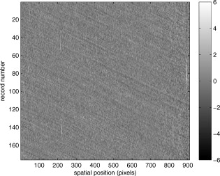
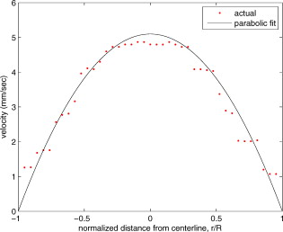
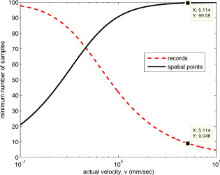
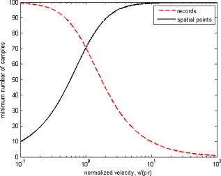
1. Introduction

There are a number of techniques for estimating blood flow velocity in the eye. One can generally categorize these techniques as being either point measurements or full-field measurements. Of the former category is laser doppler velocimetry (LDV)¹ using crossed laser beams, Doppler optical coherence tomography (OCT),^{2, 3} and adaptive optics scanning laser ophthalmoscopy (AOSLO).⁴ Of the latter category, there are imaging-based techniques using incoherent or coherent illumination as in laser speckle contrast imaging (LSCI)⁵ and its many variants.⁶ Recently, some work has been done at correlation-based tracking individual red blood cells,^{7, 8} and the so-called spatiotemporal image correlation spectroscopy.^{9, 10} Each of the above-mentioned techniques has its particular advantages and limitations. For example, OCT measures the axial component of the velocity vector (∝ cosine of the angle between the A-scan direction and the velocity vector). Although this measurement technique also captures a three-dimensional description of the vasculature, and the cosine effect could in principle be compensated for, the accuracy of this approach in vivo has not been demonstrated in the literature. The difficulty of extracting quantitative velocity estimates using laser speckle contrast techniques has been discussed by Duncan and Kirkpatrick.¹¹ Although some progress has been made recently⁵ in establishing a flow decorrelation time, the issue of relating this time constant to the flow velocity remains. At this point, in the absence of a calibration procedure, no quantitative LSCI measurements have been demonstrated. Finally, approaches based on correlation matching^{4, 7, 8, 9, 10} are clearly limited to the very smallest vessels and imaging resolutions capable of distinguishing individual red blood cells.

Although conventional crossed laser beam LDV systems are capable of characterizing three-dimensional vector velocity, these systems are quite costly and provide only real-time, pointwise measurements. The data provided are the velocities. There are no data that can be reprocessed at a later date to provide additional velocity estimates.

Herein, we detail a new approach that is related to the red blood cell tracking approach but much simpler to implement. It is based on illumination in the green wavelengths, where hemoglobin is highly absorbing, and imaging with a high-speed CCD camera. This approach, which is capable of dealing with very low signal-to-noise ratios, relies on tracking the nonuniform distribution of red blood cells within the vessel, rather than the individual blood cells themselves.

The technique extracts the gray-level values along the centerline of a vessel and stacks these traces from a sequence of images into a spatiotemporal matrix that we call a trace history. Illumination variations and noise associated with synchronization irregularities are estimated and subtracted from the trace history. The resulting residual trace history displays subtle corrugations that are associated with motion of red blood cell nonuniformities between successive frames. The actual velocity is encapsulated in the slope of these corrugations. A Radon transform is used to estimate the orientation of these corrugations and subsequently calculate the velocity. In the material that follows, we detail the theory of the concept, illustrate its performance with an in vitro study, and finish with an analysis of some typical imagery acquired with a modified fundus camera. A detailed error analysis is described that allows estimation of confidence intervals for the velocity estimates.

2. Theory and Results

All data were acquired with a modified fundus camera, which was developed for an ongoing clinical study of the etiology of diabetic retinopathy. We first describe the relevant aspects of the camera [the Johns Hopkins flow and oxygenation system (JHFOS)],¹² discuss the theory of operation in the context of a series of in vitro experiments using blood flowing through a capillary tube, and follow up with a presentation of some typical results in a human eye.

2.1.

Data Acquisition

The JHFOS was implemented by modifying a fundus imaging system (Zeiss FF3, Jena, Germany), where the original white-light source was replaced with a LED-based light engine (Enfis, Swansea, UK) centered at $525 nm$ ( $15 nm$ FWHM). The wavelength was chosen because the high absorption of both oxygenated and deoxygenated hemoglobin in that region of the spectrum allows for high contrast imaging of retinal blood vessels. An $8 -bit$ monochrome CCD imaging system (Dalsa Genie, Billerica, Massachusetts), was combined with a zoom lens with focal length of $150 - 450 mm$ , $f / 5.6 - f ∕ 3.2$ , (Computar, Commack, New York) and connected to the fundus system replacing the original film camera. The camera strobe port was used to pulse the light engine; strobe duration could be controlled programmatically and was as low as $3 μ s$ . Generally, a strobe duration of $6 μ s$ combined with a $0.5 - μ s$ strobe delay was used for the assessment of flow, hence for each captured image, the retina was illuminated for $5.5 μ s$ . Image capture was at a rate of $60 Hz$ , and integration time was the same as the strobe duration. During focusing and positioning of the system, the strobe duration was reduced to $3.0 μ s$ and the camera gain was set to maximum $(Gain = 26)$ to optimize image quality. During acquisition the gain was reduced to a lower value $(Gain = 16)$ but the strobe duration was increased to the aforementioned $5.5 - μ s$ level. This was done for two purposes. First, shorter light pulses were easily bearable by most patients during the lengthy $(\sim 5 \min)$ focusing and positioning phase; second, the lower gain setting during image acquisition allowed for a higher signal-to-noise ratio (SNR). Both camera and light engine were controlled through a custom-made software and user interface (Matlab^®, MathWorks, Natick, Massachusetts); image acquisition could be started either through the graphical user interface or by pressing a push pedal connected to a data acquisition card (National Instruments, Austin, Texas). Four seconds of images were captured for the flow analysis, and all images were saved in an uncompressed AVI format.

2.2.

In Vitro Measurements

Figure 1 illustrates a single video frame from the in vitro measurements. The vessel, a Teflon^® tube of inner diameter $165 μ m$ (object plane pixel size $7.86 μ m$ ), was positioned inside an eye phantom that mimics the optics of the human eye.¹³ The capillary tube was connected to a syringe pump (Hamilton, Reno, Nevada), and the pump rate could be adjusted to different values. For this study, flow rates of $50 μ l ∕ h$ to several hundreds were used. The box indicates the region selected for subsequent analysis. Shown in Fig. 2 is this subregion along with the calculated vessel centerline. From each video frame, we extract the gray-level values along the indicated centerline and collect them in the form of a spatiotemporal matrix, which we call a trace history, as illustrated in Fig. 3 . We denote this trace history simply as $g (t_{i}, d_{j})$ , where $t_{i}$ is time (here in terms of the record number, where $1 ⩽ i ⩽ N_{t}$ , and $N_{t}$ is the number of records), and $d_{j}$ is distance along the centerline (here in pixels, where $1 ⩽ j ⩽ N_{s}$ , and $N_{s}$ is the number of pixels along the centerline). There are a number of features visible in such a display. As seen in Fig. 1, the effective illumination varies over the field (a combination of camera vignetting and nonuniform illumination). As a result, the illumination along the horizontal direction of Fig. 3 is seen to vary. Additionally, there are occasional noisy data that are reflected in discontinuous records. Superimposed on these illumination variations is a mottled appearance wherein lies the information on blood velocity.

Fig. 1

Single video frame of blood-filled vessel with region for subsequent analysis indicated.

Fig. 2

Vessel with specified centerline.

Fig. 3

Spatiotemporal display, the “trace history,” of centerline gray levels.

To eliminate the illumination variations, we calculate the following means from the trace history of Fig. 3:

Eq. 1

\bar{g} (t_{i}) = \frac{1}{N_{s}} \sum_{j} g (t_{i}, d_{j}); \bar{g} (d_{j}) = \frac{1}{N_{t}} \sum_{i} g (t_{i}, d_{j}); \bar{g} = \frac{1}{N_{s} N_{t}} \sum_{i} \sum_{j} g (t_{i}, d_{j}) .

Here,

\bar{g} (t_{i})

is a vector of length

N_{t}

and

\bar{g} (d_{j})

is a vector of length

N_{s}

. From these two vectors, we form the outer product

Eq. 2

\hat{g} = \frac{\bar{g} {(d_{j})}^{t} \bar{g} (t_{i})}{\bar{g}},

which is illustrated in Fig. 4 . One observes that Fig. 4 displays the illumination variations associated with Fig. 3, but none of the mottled appearance. Finally, Fig. 5 shows the residual of this illumination-compensated gray-level trace history,

Eq. 3

r (t_{i}, d_{j}) = \frac{g (t_{i}, d_{j})}{\hat{g} (t_{i}, d_{j})} - \frac{1}{N_{s} N_{t}} \sum_{i} \sum_{j} \frac{g (t_{i}, d_{j})}{\hat{g} (t_{i}, d_{j})} .

The values of this residual represent the gray-level variations about the illumination-compensated trace history. As shown here, values of this residual are typically on the order of plus or minus six gray levels.

Fig. 4

Illumination level estimated from Fig. 3 [see Eq. 2].

Fig. 5

Residual of illumination-compensated trace history [see Eq. 3].

Figure 5 displays a mottling appearance that is a reflection of the blood cell motion along the centerline of the vessel. Specifically, the tilt of the corrugated structure corresponds to the motion, from one video frame to the next, of the nonuniform distribution of red blood cells. We generate an estimate of this tilt from the Radon transform as illustrated in Fig. 6 . Figure 6 is the Radon transform of the illumination-compensated residual trace history shown in Fig. 5. Note the structure in the projection (arrow). Subsequently, we calculate the SNR in the projection at each angle (see Fig. 7 ). We define this as the quotient of the root-mean-square (RMS) variation in the projection at a specific angle to the rms variation in the entire trace-history residual image,

Eq. 4

SNR = \frac{σ_{R} (θ)}{σ_{I}} .

This parameter is effectively a measure of the amount of deterministic structure in the projection at a given projection angle. In Fig. 7, the peak corresponds to the orientation of the tilted structure in the residual trace history. The 90% levels are used to determine an uncertainty interval. The slope is in units of records per pixel; to convert to velocity, we use

Eq. 5

v = p \cdot r ∕ m,

where

p

is the object plane pixel size,

r

is the frequency at which the records are acquired, and

m = \tan θ

is the slope of the structure. The velocity uncertainty interval is computed in an identical fashion. Note that the slope of the corrugated structured can be either positive or negative. Thus, flow direction is readily determined.

Fig. 6

Radon transform of illumination-compensated trace history residual shown in Fig. 5. The projection angle is positive in the counterclockwise direction from the $y$ -axis ( $- 90 \deg$ represents a zero slope). Note peak projection value (arrow).

Fig. 7

RMS power in the projection at each angle [see Eq. 4].

One other feature of the SNR plot shown in Fig. 7 is the null at the $- 90 - \deg$ projection angle. This angle, which corresponds to zero velocity, is the projection of the trace-history residual along the spatial axis (i.e., a sum over the columns). The specific illumination compensation algorithm that we use guarantees that this projection value be zero.

All the discussion thus far has been devoted to flow-velocity estimation along the centerline. In fact, our software is designed to specify this centerline. Once specified, however, it is a simple matter to identify a parallel line displaced from the centerline. In this manner, the velocity profile can be explored. An example of such a calculation for the in vitro model previously discussed is shown in Fig. 8 . Also shown in Fig. 8 is the parabolic fit to the measured data. Using the relationship $Q = v_{\max} π R^{2} ∕ 2$ leads to a volume flow rate estimate of $196 μ l ∕ h$ . The 15% discrepancy from the purported pump flow rate of $170 μ l ∕ h$ is well within the pump flow rate uncertainty. Volume flow estimates such as this are of vital interest in establishing perfusion.

Fig. 8

Velocity profile for in vitro flow model (points) and least squares parabolic fit (line).

2.3.

Error Analysis

To explore the determining factors in the accuracy of the velocity estimate, we acquired a large residual trace history and computed Radon transforms, and thus velocities estimates, on various subsets of the data. Figure 9 illustrates the variables of concern. In Fig. 9 we illustrate the maximum length of the sequence of data points, $l_{p}$ , over which the projection is computed. The length of this sequence is of interest because it affects the SNR of the resulting Radon transform. Note that the Radon transform simply sums elements along various directions. It is only in certain summation (projection) directions that the structure due to the moving red blood cells will appear consistently. It is also reasonable to assume that the trace history residual contains zero mean Gaussian white noise. Analysis of the background surrounding the vessel has shown that this is indeed the case. As such, in the particular summation direction, the signal will contain a signal (the consistent structure) as well as additive noise. The summation will thus result in a SNR gain in proportion to the square root of the number of elements in the summation. The longer the element, $l_{p}$ , is, the larger the SNR gain is. This length obviously depends on the number of records, the number of pixels, and the angle of the structure,

Eq. 6

l_{p} = \min (\frac{N_{s}}{\cos θ}, \frac{N_{t}}{\sin θ}) .

Figure 10 is the result of this analysis. Also shown in Fig. 10 is the power law fit

Eq. 7

e = 1.09 l_{p}^{- 0.5} .

The

- 1 ∕ 2

power law is to be expected for the standard deviation of a sequence of independent Gaussian distributed samples. With a threshold criterion on the velocity uncertainty, one can choose the appropriate length of the time sequence and the distance along the centerline,

8.

1.09 l_{p}^{- 0.5} ⩽ e_{o},

l_{p} ⩾ {(\frac{1.09}{e_{o}})}^{2} \approx \frac{1}{e_{o}^{2}},

\min (\frac{N_{s}}{\cos θ}, \frac{N_{t}}{\sin θ}) ⩾ \frac{1}{e_{o}^{2}},

but from Eq. 5, we have

\tan θ = \frac{p r}{v},

and thus,

Eq. 9

\sin θ = \frac{p r}{\sqrt{v^{2} + {(p r)}^{2}}}; \cos θ = \frac{v}{\sqrt{v^{2} + {(p r)}^{2}}},

so that finally,

Eq. 10a

\sqrt{v^{2} + {(p r)}^{2}} \min (\frac{N_{s}}{v}, \frac{N_{t}}{p r}) ⩾ \frac{1}{e_{o}^{2}}

or

Eq. 10b

\min (N_{s}, \frac{N_{t}}{p r ∕ v}) ⩾ \frac{1}{e_{o}^{2} \sqrt{1 + {(p r ∕ v)}^{2}}} .

The values of

N_{s}

and

N_{t}

satisfying this inequality are show in Fig. 11 . As an example, for the modal angle of

θ = 5.19 \deg

, the velocity estimate for the centerline flow is

5.12 mm ∕ s

. For these measurements,

p \cdot r = (0.165 mm) (60 Hz) = 0.465 mm ∕ s

so that

p r ∕ v = 0.0908

. If we want a velocity uncertainty of no more that 10%, then we require

11.

\frac{p r ∕ v}{e_{o}^{2} \sqrt{1 + {(p r ∕ v)}^{2}}} = 9.096 ⩽ N_{t},

\frac{1}{e_{o}^{2} \sqrt{1 + {(p r ∕ v)}^{2}}} = 99.59 ⩽ N_{s} .

We can satisfy these requirements with 10 records

(\sim 0.17 s)

and 100 spatial samples

(\sim 0.79 mm)

. Figure 12 shows the required number of spatial and temporal samples as a function of velocity for the current system, where

p \cdot r = (7.86 μ m) (60 Hz) = 0.472 mm ∕ s

. Figure 13 is in terms of normalized velocity and applicable to a generic system.

Fig. 9

Illustration of the geometric relationships among the variables in the error analysis model.

Fig. 10

Fractional uncertainty in velocity estimate as a function of projection length (points) and power law fit (line).

Fig. 11

Values of $N_{t}$ and $N_{s}$ satisfying desired inequality [see Eq. 10b].

Fig. 12

Required number of spatial and temporal samples for current system [see Eq. 11].

Fig. 13

Required number of spatial and temporal samples for generic system.

2.4.

In Vivo Measurements

Analysis of the in vivo imagery is a semi-automated process that requires an analyst to select a sequence of image frames, superimpose an analysis grid on the fundus image, and specify a region along a specific vessel for which the velocity is to be estimated. An added complication is that the image sequence must be registered prior to the calculations indicated previously. Each of these steps is illustrated in the following discussion.

For the fundus imagery, the subject eye is dilated by instilling 1% tropicamide and 2.5% phenylephrine eye drops. Fixation of the undilated eye is also sought to minimize eye movements. We typically acquire $2 s$ of data at $60 Hz$ and then screen for major saccades. The sequence of images between these major saccades is then registered by a two-step rigid-body translation. Because the image motions are typically small, a pure translation is sufficient. The first step is based on a correlation matching and achieves registration to the nearest pixel. The subsequent registration, based on a gradient technique,^{14, 15, 16} registers to a subpixel precision. The registration process is initialized by the analyst selecting a region of the fundus image on which to base the registration process. Typically, a region displaying a good deal of vasculature is chosen (see Fig. 14 ). Note that the entire image at each frame is registered, but the estimates of the image shift are derived only from the specified region. From the registered set of images, a mean image is computed and displayed to the analyst. The analyst chooses a center point about which a mask is drawn (Fig. 15 ). This mask consists of a series of concentric circles of diameters 1, 2,…, $6 mm$ further subdivided into north, east, south, and west sectors. Our clinical interest is in the velocity within the vessels that cross the curves separating the various zones. To make this determination, the analyst makes an initial selection of a short segment of a vessel. Subsequent to the initial selection of the vessel, its centerline is determined through a line-growing process based on examination of the distance between a specific pixel and the vessel walls. See Appendix { label needed for app[@id='x0'] }for a discussion of this vessel centerline specification algorithm.

Fig. 14

Region of image from which registration estimates are to be derived. Object plane pixel size is $6 μ m$ .

Fig. 15

Fundus image with superimposed mask and selected vessel segment. Circle diameters are 1, 2, 3, 4, 5, and $6 mm$ . Flow velocities for venules (V) and arteries (A) indicated in millimeters per second. The occasional light-colored spots are caused by dust on imaging lens.

Some typical results are shown in Fig. 15. For this analysis, 20 records $(\sim 0.3 s)$ of data were used. The marked image improvement between Figs. 14 and 15 is due to the averaging over the 20 frames. Some typical results for venous (V) and arterial (A) flow are displayed in millimeters per second. As expected, the velocities in the daughter vessels (whether venous or arterial) are lower than in the parent. Direct comparison between arterial and venous velocities cannot be made at this point because the vessels are of various sizes and we have not yet accounted for this factor.

3. Discussion and Conclusions

Interestingly, the concept of what we call a trace history has arisen previously. For example, in the context of tracing individual erythrocytes within capillary networks, Jensen and Gluckberg¹⁷ derived such a spatiotemporal matrix but did not use it for other than display purposes. Zhong, ⁴ using a modified AOSLO, also derived such a spatiotemporal display, which they called an XT image. Zhong ⁴ derived velocity estimates based on the slope of the structures in the XT images, but their processing approach was not discussed in detail.

For the in vitro studies, the trade-offs involved in selecting the required number of records and length of trace were clear cut. For the in vivo imagery, there is the added complication that the velocities are generally pulsatile in nature. As a result, we have the added restriction that the time over which the sequence of exposures is acquired must be small compared to the period of the pulse. Under the assumption of no a priori information on the pulse period, it must be measured. We have demonstrated that this pulse period can be established through observation of the temporal variations in speckle contrast.¹⁸ In future work, this factor will be incorporated into the velocity estimation algorithm.

One aspect of this approach that is critical is the compensation for illumination variations. The outer product formed from the row and column means of the trace history is particularly effective at removing these multiplicative effects. Implicit in this approach is that the illumination variations are independent in the two Cartesian dimensions of the trace history (time and space). There are other approaches that could be used, such as Fourier filtering or even singular value decomposition,¹⁹ but the outer product is particularly effective at capturing the a priori knowledge of independence in the two domains. Nevertheless, we continue to explore other noise-removal strategies.

A reoccurring criticism of Doppler measurements of whatever kind is that velocity does not equal flow. Although this is true, they are in fact highly correlated. For example, for flow of a Newtonian fluid within a vessel, the velocity profile is parabolic (Poiseuille flow). As a result, the volume flow can be inferred from a measurement of the centerline velocity. Blood, however, is non-Newtonian; at low shear rates, it displays an elevated viscosity attributed to the agglomeration of cells, while at high shear rates the lowered viscosity is attributed to deformation of cells.²⁰ Nevertheless, a number of studies^{21, 22, 23} suggest that for vessels between 155 and $2000 μ m$ , the effect can be ignored. As a result, a measurement of centerline velocity together with knowledge of the configuration of the vessel can be used to infer volume flow rate.

Not discussed previously, but merely alluded to, was the mechanism by which the flow manifests itself. For the resolution of our modified fundus camera, the individual red blood cells are not resolvable. It is commonly accepted, however, that the red blood cells are not evenly distributed but aggregate into structures known as rouleaux²⁰ because of the resemblance to stacks of coins. It is perhaps these aggregates that are responsible for the structure observed in the trace histories. Moreover, we have implicitly assumed that this organizational structure moves along the vessel en masse. This is much akin to Taylor’s “frozen turbulence” hypothesis²⁴ used in the treatment of propagation through turbulence. This loss of organizational coherence obviously affects the choice of optimum trace length and record number. This coherence effect can be observed in the residual trace history, particularly for low flow velocities, but has yet to be quantified.

An important issue yet to be explored is the size of vessels within which we can estimate flow. The ultimate limit is dictated by resolution and contrast (these factors also influence the accuracy of the centerline specification algorithm). Additionally, the choice of wavelength and the resulting absorption depth for hemoglobin has an impact on how deeply we see into the vessel. At the smallest vessel diameters, however, the concept of absorption depth loses its meaning; one may be observing individual RBCs at this point.

Finally, the range of velocities that are measurable with this technique have not been discussed. Clearly, as the flow velocity approaches zero, the orientation of the corrugated structure seen in Fig. 5 will approach the vertical. This structure thus will become indistinguishable from the noise associated with nonuniform illumination. The question remains as to how large the inclination angle can be before the signal structure becomes lost in the noise. In the other extreme, the inclination angle will approach the horizontal axis. Thus, the structure associated with nonuniform distribution of blood cells will disappear into the noise associated with camera/strobe timing errors. Each of these limits is expressible in terms of the SNR of the measurement, and the exact relationships remain to be established.

From these comments, it is clear that there are many avenues for improving and exploiting this measurement concept. It is further evident, however, that this approach, which entails rather minor modifications to existing fundus cameras, constitutes a valuable tool for quantitative assessment of ocular blood flow.

We are currently conducting a clinical trial using our modified fundus camera, the JHFOS.¹² To date, we have measured 106 individuals with varying stages of diabetic retinopathy in comparison to subjects with no known ocular diseases except refractive errors. Results of the trial will be published shortly.

Appendices

{ label needed for app[@id='x0'] }

Appendix

Here we provide some of the details of the algorithm for determining vessel centerlines. The process is illustrated with a single frame from the in vitro measurements (Fig. 16 ). The centerline calculation starts with the manual placement of points A and B in Fig. 16 by the analyst. Point A determines the approximate starting point for the centerline and B, the approximate end point. Image preprocessing steps are applied to the highlighted area to remove the effects of variable illumination levels. Typically, we use a least-squares fit cubic polynomial surface.

Fig. 16

Illustration of pixel selection to initiate centerline determination algorithm.

Measuring the distance of a pixel to the border of the blood vessel is achieved by using an iterative process that begins with a composite +× pattern. At each iteration, a single pixel is added to each of the eight end points of the pattern. This process continues until the gray-level value of one outer pixel of a line reaches a threshold value. This determines that the pixel at the end of the pattern is outside of the blood vessel. Thus, the number of iterations performed by the algorithm corresponds to the distance of the pixel to the vessel border.

The distance of every pixel to any vessel border is calculated for pixels in proximity to the selected point, A and the local maximum is chosen as starting point for the further centerline calculation. The next pixel of the centerline is the local distance maximum of all pixels that are adjacent to the starting point; every following pixel is calculated accordingly.

Under the constraint that a pixel must not be adjacent to any centerline pixel except the most recent one, it is ensured that the centerline moves straightforward; a comparison of tangent vectors is used in case there is no distinct maximum for the choice of the next pixel. The area around the selected pixel B determines the break condition for the growing process.

Acknowledgment

This work was sponsored in part by National Institutes of Health Grant No. RO1 EY017577.

References

1.

F. Durst, A. Melling, and J. H. Whitelaw, Principles and Practice of Laser-Doppler Anemometry, 2nd ed.Academic Press, London (1981). Google Scholar

2.

R. K. Wang and L. An, “Doppler optical microangiography for volumetric imaging of vascular perfusion in vivo,” Opt. Express, 17 8926 –8940 (2009). https://doi.org/10.1364/OE.17.008926 1094-4087 Google Scholar

3.

R. Wang, L. An, and D. Wilson, “Visualizing ocular perfusion with optical microangiography,” (2010) http://dx.doi.org/10.1117/2.1201002.002571 Google Scholar

4.

Z. Zhong, B. L. Petrig, X. Qi, and S. A. Burns, “In vivo measurement of erythrocyte velocity and retinal blood flow using adaptive optics scanning laser ophthalmoscopy,” Opt. Express, 16 12746 –12756 (2008). https://doi.org/10.1364/OE.16.007508 1094-4087 Google Scholar

5.

A. B. Parthasarathy, W. J. Tom, A. Gopal, X. Zhang, and A. K. Dunn, “Robust flow measurement with multi-exposure speckle imaging,” Opt. Express, 16 1975 –1989 (2008). https://doi.org/10.1364/OE.16.001975 1094-4087 Google Scholar

6.

D. A. Boas and A. K. Dunn, “Laser speckle contrast imaging in biomedical optics,” J. Biomed. Opt., 15 011109 (2010). https://doi.org/10.1117/1.3285504 1083-3668 Google Scholar

7.

D. A. Nelson, S. Krupsky, A. Pollack, E. Aloni, M. Belkin, I. Vanzetta, M. Rosner, and A. Grinvald, “Special report: noninvasive multi-parameter functional optical imaging of the eye,” Ophthal. Surg. Lasers Imaging, 36 57 –66 (2005). Google Scholar

8.

D. Izhaky, D. A. Nelson, Z. Burgansky-Eliash, and A. Grinvald, “Functional imaging using the retinal function imager: direct imaging of blood velocity, achieving fluorescein angiography-like images without any contrast agent, qualitative oximetry, and functional metabolic signals,” Jpn. J. Ophthalmol., 53 345 –341 (2009). https://doi.org/10.1007/s10384-009-0689-0 0021-5155 Google Scholar

9.

B. Hebert, S. Costantino, and P. W. Wiseman, “Spatiotemporal image correlation spectroscopy (STICS) theory, verification, and application to protein velocity mapping in living CHO cells,” Biophys. J., 88 3601 –3614 (2005). https://doi.org/10.1529/biophysj.104.054874 0006-3495 Google Scholar

10.

M. Rossow, W. W. Mantulin, and E. Gratton, “Spatiotemporal image correlation spectroscopy measurements of flow demonstrated in microfluidic channels,” J. Biomed. Opt., 14 024014 (2009). https://doi.org/10.1117/1.3088203 1083-3668 Google Scholar

11.

D. D. Duncan and S. J. Kirkpatrick, “Can laser speckle flowmetry be made a quantitative tool?,” J. Opt. Soc. Am. A, 25 2088 –2094 (2008). https://doi.org/10.1364/JOSAA.25.002088 0740-3232 Google Scholar

12.

J. C. Ramella-Roman, S. A. Mathews, H. Kandimalla, A. Nabili, D. D. Duncan, S. A. D’Anna, S. M. Shah, and Q. Nguyen, “Measurement of oxygen saturation in the retina with a spectroscopic sensitive multi aperture camera,” Opt. Express, 16 6170 –6182 (2008). https://doi.org/10.1364/OE.16.006170 1094-4087 Google Scholar

13.

P. Lemaillet and J. C. Ramella-Roman, “An eye phantom for measurement of retinal oxygenation,” J. Biomed. Opt., 14 (6), 064008 (2009). https://doi.org/10.1117/1.3258669 1083-3668 Google Scholar

14.

J. M. Fitts, “Precision correlation tracking via optimal weighting functions,” 280 –283 (1979). Google Scholar

15.

L. Stephan, J. E. Albus, and J. Marcovici, “Fitts correlation tracker fidelity in presence of target translation, rotation, and size change,” Proc. SPIE, 4714 196 –207 (2002). https://doi.org/10.1117/12.472594 0277-786X Google Scholar

16.

S. Wong, “Advanced correlation tracking of objects in cluttered imagery,” Proc. SPIE, 5810 158 –169 (2005). https://doi.org/10.1117/12.598647 0277-786X Google Scholar

17.

P. S. Jensen and M. R. Gluckberg, “Regional variation in capillary hemodynamics in the cat retina,” Invest. Ophthalmol. Visual Sci., 39 407 –415 (1998). 0146-0404 Google Scholar

18.

D. D. Duncan, S. J. Kirkpatrick, J. C. Gladish, and S. A. Hurst, “Laser speckle contrast imaging for the quantitative assessment of flow,” Proc. SPIE, 7176 717603 (2009). https://doi.org/10.1117/12.809401 0277-786X Google Scholar

19.

G. H. Golub and C. F. Van Loan, “Matrix Analysis,” Matrix Computations, Third ed.Johns Hopkins University Press, Baltimore (1996). Google Scholar

20.

P. Vennemann, R. Lindken, and J. Westerweel, “In vivo whole-field blood velocity measurement techniques,” Exp. Fluids, 42 495 –511 (2007). https://doi.org/10.1007/s00348-007-0276-4 0723-4864 Google Scholar

21.

S. E. Charm and G. S. Kurland, “On the significance of the Reynolds number in blood flow,” Biorheology, 3 (3), 163 –164 (1966). 0006-355X Google Scholar

22.

S. E. Charm, G. S. Kurland, and S. L. Brown, “The influence of radial distribution and marginal plasma layer on the flow of red cell suspensions,” Biorheology, 5 (1), 15 –43 (1968). 0006-355X Google Scholar

23.

S. E. Charm and G. S. Kurland, Blood Flow and Microcirculation, Wiley, Hoboken, NJ (1974). Google Scholar

24.

J. W. Goodman, Statistical Optics, Wiley, Hoboken, NJ (1985). Google Scholar

Citation Download Citation

Donald D. Duncan, Paul Lemaillet, Mohamed Ibrahim, Quan Dong Nguyen, Matthias Hiller, and Jessica Ramella-Roman "Absolute blood velocity measured with a modified fundus camera," Journal of Biomedical Optics 15(5), 056014 (1 September 2010). https://doi.org/10.1117/1.3494565

Published: 1 September 2010

Access the abstract

JOURNAL ARTICLE
8 PAGES

DOWNLOAD PAPER SAVE TO MY LIBRARY

GET CITATION

CITATIONS

Cited by 30 scholarly publications.

Explore citations on Lens.org

RIGHTS & PERMISSIONS

Get copyright permission Get copyright permission on Copyright Marketplace

KEYWORDS

Blood

Cameras

Velocity measurements

Error analysis

Signal to noise ratio

In vitro testing

Radon transform

1.

Introduction

2.

Theory and Results