
|
|
1.IntroductionElectrophysiological investigations of the visual system are well established in clinical practice and research. Important methods in such investigations include the electroretinogram (ERG), the visual evoked potential (VEP), and the electrooculogram, 1, 2 which employ stimulation with temporal, spatial, and chromatic paradigms. 3, 4 The silent substitution technique (SST) is suitable for chromatic stimulation and provides selective excitation of the three cone types. 5, 6 The SST has become a wide variety of applications in the fields of ophthalmic and vision science. 7, 8, 9, 10, 11, 12 Imaging of the human retina is another essential tool for medical diagnosis. Fundus cameras reveal anatomical surface information, while optical coherence tomography (OCT) is widely used to investigate 3-D morphologic changes and blood flow velocities. 13, 14, 15, 16 In addition, polarimetry techniques, such as scanning laser polarimetry, have been developed to selectively analyze the different layers of the retina. 17, 18, 19 In a previous study, we implemented the SST using a circular flash stimulation, presented on a 30–in. liquid-crystal display (LCD) stimulator, to excite short-, medium-, and long-wavelength-sensitive cones (S-, M-, and L-cones). On the basis of the obtained VEPs, we were able to detect glaucoma and objectively determine its severity.20 However, the major drawbacks of common electrophysiological examination methods are the inability to reveal the exact stimulus position on the retina and the absence of information about the individual fundus morphologies related to the area of stimulation. Thus, stimulus placement based on structures under investigation as well as pathological findings (e.g., glaucomatous or age-related macular degeneration) is not possible. Furthermore, the effects of fixation problems and eye movements cannot be fully addressed with current standard technologies. As a result, the diagnostic significance is limited or maybe reduced. To overcome such insufficiencies, we designed a new fundus-controlled stimulation setup that current clinical practice lacks. In this context, control means performing fundus imaging, projecting defined stimuli (position, shape, size, color) onto the retina, as well as fundus-based real-time monitoring of the mentioned stimuli parameter. In this paper, we present a novel optoelectrophysiological setup that combines optical imaging, functional stimulation, and electrophysiological investigation. Therefore, we connected a digital color liquid crystal on silicon (LCoS) projector, an electron-multiplying imager, and a light-emitting diode to a fundus camera. We comprehensively characterized the properties of the designed stimulator and demonstrated its functionality by presenting electroencephalographic (EEG) measurements. Compared to common stimulation methods and devices, this developed setup has the advantage to perform electrophysiological examination of the visual system, and selective color channel stimulation in particular, under fundus-controlled conditions. Consequently, the information gap concerning the individual fundus morphologies and the exact stimulus position on the fundus can be closed. 2.Methods2.1.SubjectsWe studied six randomly selected healthy male volunteers (age, 25–30 years). All subjects were free of ocular diseases, had visual acuities between 0.8 and 1.0, and their color vision was tested with Ishihara and Stilling-Velhagen plates. The tests revealed no color vision abnormalities. None of the volunteers had a history of neurological or psychological disorders, and none was taking any medication or drugs. The subjects had excellent target fixation and demonstrated normal saccadic behavior. After receiving an explanation of the details and the purpose of the study, all the subjects gave their informed consent. All experiments were conducted in accordance with the Declaration of Helsinki. 2.2.StimulatorA suitable projector unit was selected for the fundus-controlled projection stimulator, which should be capable of producing SST chromatic stimuli. On the basis of the resolution, pixel pitch, aperture ratio, electro-optical response times, channel cross talk, and line flickering (Table 1), we chose a three-panel micro LCoS (3LCoS) projector (ASI6001-01, Aurora Systems, San Jose California). This projector was connected to the examination and stimulation unit (THERA PRAX system, neuroConn GmbH, Ilmenau, Germany) via a digital visual interface (DVI). The unit generates stimulations and records EEG data. Fig. 8PA versus central stimulation within the MA. (a) Corresponding stimulation areas containing (top) MA and (bottom) PA. (b) S-cone responses and (c) LM-cone responses. All responses are from electrode Oz.  Table 1Parameters of the three-chip micro LCoS projector (ASI6001-01).
The electro-optical response time depends on the gray-scale value, respectively, the color value of the image. For SST stimulation, this produces a finite time difference between the start and end points of the presented color combination, which can cause contrast losses and distortions of the VEPs. The stimulator LCoS electronics must have a sufficiently large temporal bandwidth to achieve the desired maximum stimulus contrast. To analyze the contrast losses, we measured the temporal modulation transfer function (tMTF) using a PIN photodiode (BPX 65, Siemens, Munich, Germany). This photodiode was placed in the focal plane behind an artificial eye lens model (1177-617, Carl Zeiss Meditec, Jena, Germany) to simulate the target area of stimuli for a human retina. We detected the signal amplitude of the diode by increasing the flicker frequency in steps of the corresponding frame time. At each frequency, the average of 100 amplitude values was calculated. The computed standard deviation was <0.6% of the mean. We measured the tMTF for black−white flickering and for the color combinations for S-cone stimulation and LM-cone stimulation. An additional problem is the frame delay generated by the LCoS electronic interface. It takes a certain time to convert the video signal into the LCoS driver signal. To correct this effect in the EEG, we used the same photodiode and analyzed its signal and a synchronization trigger from the stimulation unit. The trigger coincided with the onset of stimulus generation, while the photodiode signal coincided with stimulus imaging by the projector. Signal analysis was performed using a digital oscilloscope (TDS 3054, Tektronix, Beaverton, Oregon). We also verified the LCoS refresh rate of 60 Hz with the same instrumentation by applying a 30-Hz flicker sequence generated by the stimulation system. We used a fundus camera (VISUCAM lite, Carl Zeiss Meditec, Jena, Germany) to overcome the problems of stray light, direct reflections, and ghost reflections in the eye and in the instrument optics. To image chromatic SST stimuli onto the fundus, the 3LCoS projector was inserted in the illumination path of the fundus camera utilizing additional optics for the coupling. This created a new optical path, which is herein referred to as the stimulation path. Real-time fundus imaging and control could be achieved using the existing fundus camera port of the observation path. An intermediate fundus image produced by the ophthalmoscope lens is projected by a second lens onto a digital imager. The imager was connected to a control unit, which allows the observer to react on fundus conditions. To evaluate the optimal image quality, we performed sensitivity tests with three digital camera systems (see Section 2.4). The dependence of the spatial performance on LCoS resolution and the optics was analyzed using the spatial modulation transfer function (sMTF). This was carried out for the stimulation path using the primary colors of the projector. We generated an incoherent image of a nearly ideal razor blade edge. The sMTF could be obtained by edge differentiation and then taking the Fourier transformation.21 Finally, we selected a projector light source. We used a high-power light emitting diode (LED) (OSTAR LE UW E3B, Osram, Munich, Germany) that has a smooth spectrum and emits high energy at lower wavelengths. The output spectra of the primary colors did not overlap due to the optimized dichroic layers in the LCoS core. The LED offers a luminous flux of up to 1120 lm and a white point with the CIE 1931 color coordinates x = 0.31 and y = 0.32. We used a cooling element to stabilize the diode temperature. The entire fundus-controlled LCoS projection stimulator is depicted in Fig. 1. Fig. 1(a) Optical schematic of the fundus-controlled LCoS projection stimulator. (b) The LCoS projection stimulator without housing. The stimulation path consists of the following components: light source (LED) with cooling element and optics (L1) that collimates the LED light (LO); three-channel (RGB) LCoS core (3LCoS); coupling optics (CO) with lenses (L2 and L3) to image the generated stimuli into the fundus camera (FC) and stop (S1) to form the entrance pupil of the FC; lenses (L4 and L5) and ophthalmoscope lens (OL) to image the stimuli onto the fundus; pinhole mirror (PM), which enables both simultaneous stimulation and control; and stop (S2), which is conjugate to the fundus, and limits its field of view. The observation path of the camera consists of the following components: ophthalmoscope lens (OL) to produce an intermediate image of the fundus (IF), PM, and lens (L) to project the fundus image onto the camera detector (EMCCD). The control unit (CU) displays the stimulation target area (TA) and the fundus, enabling adjustments to be made based on individual conditions. The stimulation unit (SU) is connected to the LCoS projector and controls the SST stimuli. EEG recording is not shown in this schematic.  2.3.Energy AdjustmentTo compare the measured VEPs to the data from our previous study, we adjusted the maximum light output of the LCoS projector. This working point calibration was performed by considering the full white spectra of the projector and the previous stimulator system (30–in. LCD stimulator). The adjustment is based on a radiometric parameter: the radiant flux Φe_p in the plane of the pupil. For the LCD, we computed the flux using the following equation: Eq. 1[TeX:] \documentclass[12pt]{minimal}\begin{document}\begin{equation} \Phi _{{\rm e\_p}} = E_{{\rm e\_p}} A{}_{\rm p}(L_{\rm e}), \end{equation}\end{document}Eq. 2[TeX:] \documentclass[12pt]{minimal}\begin{document}\begin{equation} d_{\rm p} = 1.29 + \frac{{6.62}}{{1 + \left({L_{\rm e} /8.24} \right)^{0.32} }}. \end{equation}\end{document}To compare the VEPs generated from different stimulator systems, the retina irradiances (E e_r) must be equal in all cases. Using the value of E e_r for our LCD stimulator, we computed Φe_p as a set point of the LCoS projector. The retina area was obtained from the maximum projector target area of the stimuli and the geometry of Gullstrand's eye model. The computed radiant flux for adjusting the LCoS projector was 0.63 mW. This adjustment was realized by inserting neutral density filters in the illumination path. 2.4.Digital Fundus ImagingTo make adjustments based on the condition of a patient's fundus, a high-quality image is important for controlling and positioning the SST stimuli on the retina. We performed sensitivity tests with three different camera systems: a complementary metal-oxide-semiconductor (CMOS) camera (Guppy F-036C, Allied Vision Technologies, Stadtroda, Germany), a charge-coupled device (CCD) camera (CF 8/5 MX, Kappa opto-electronics GmbH, Gleichen, Germany), and an electron-multiplying CCD (EMCCD) camera (Luca R 604, Andor Technology PLC, Belfast, United Kingdom). The main parameters that affect the sensitivity are listed in Table 2. Table 2Parameters of the tested camera systems.
The sensitivity was analyzed by varying the irradiance as the input signal and detecting the image gray value as the response signal. To illuminate the different imagers homogenously, we used the stimulation path of the stimulator and a barium-sulfate-coated integrating sphere (K-100W, LOT-Oriel GmbH, Darmstadt, Germany) was placed directly in front of the imagers. To enable the results to be compared, the CMOS imager was used in monochromatic mode and the cameras were set to an exposure time of 100 ms. We performed all measurements with a gain of 0 dB, without automatic gain control and without any pixel binning. The testing process was conducted using both the full white spectrum and the green spectrum of the stimulator, and it was performed three times to evaluate reproducibility. To estimate the average gray value, a region of interest (100×100 pixels) was centered in the image. We measured the input irradiance with the radiometer in the same plane as the camera imagers. Because of the sensitivity results (see Section 3), the EMCCD system was used in the observation path. A universal serial bus interface provided the connection with the control unit. 2.5.SST StimulationAll stimuli sequences were imaged with the experimental LCoS projection stimulator. To avoid temporal and spatial distortions generated by applying interpolation algorithms to DVI input signals, we used only the native resolution of 1920×1080 pixels. The maximum target area of the stimuli on a human retina was about 27×15 deg. Image and video enhancement options were disabled, as were sharpness and noise reduction algorithms on the LCoS engine. To selectively modulate activity in the S- and LM-cone pathways, we presented two different SST flash sequences in a full field. For one volunteer, we performed papilla stimulation to estimate the influence of stray light and geometrical correctness on optical imaging. Each stimulation sequence contained two different color stimuli. The silent substitution condition was realized by alternating these colors. The two colors correspond to two states, the ON and OFF states, which are related to different cone activations. The activation can be simplified using the following instantiations: L1 = L2, M1 = M2, S1 ≠ S2 (for S-cone condition) and L1 ≠ L2, M1 ≠ M2, S1 = S2 (for LM-cone condition). The color values and the exact cone activation were calculated using the Hunt fundamentals for 10-deg and larger viewing conditions [using Eq. 4]. 24, 25 Therefore, the input red, green, and blue (RGB) values of the stimulation unit were converted into the standard color values of virtual XYZ space [using Eq. 3]. As a precondition, the spectral distribution function for the RGB channels of the stimulator were measured using a compact array spectroradiometer (CAS 140B, Instruments Systems, Munich, Germany). The time constancy of the emission spectra for all three color channels was checked to ensure that the emission levels did not vary during the SST sequences. Gamma correction was performed by determining the characteristic gamma curve for the LCoS projector and the graphics card (8 bit). The mean quantification error was 0.96% for the red channel, 0.76% for the green channel, and 0.46% for the blue channel (given as percentages of the maximum light output of each channel). The transformation matrices [Eqs. 3, 4] for the applied stimulation system are as follows: Eq. 3[TeX:] \documentclass[12pt]{minimal}\begin{document}\begin{equation} \hspace*{-30pt}M_{{\rm RGB}\to{\rm XYZ}} = \left({\begin{array}{*{20}c} {0.37} &\quad {0.34} &\quad {0.19} \\ {0.18} &\quad {0.76} &\quad {0.06} \\ {0.00} &\quad {0.02} &\quad {0.94} \\ \end{array}} \right), \end{equation}\end{document}Eq. 4[TeX:] \documentclass[12pt]{minimal}\begin{document}\begin{equation} M_{{\rm XYZ} \to {\rm LMS}} = \left({\begin{array}{*{20}c} \hphantom{-}{0.39} &\quad {0.69} &\quad { - 0.08} \\ { - 0.23} &\quad {1.18} &\quad \hphantom{-}{0.05} \\ \hphantom{-}{0.00} &\quad {0.00} &\quad \hphantom{-}{1.00} \\ \end{array}} \right). \end{equation}\end{document}Eq. 5[TeX:] \documentclass[12pt]{minimal}\begin{document}\begin{equation} \left({\begin{array}{*{20}c} {\rm L} \\ {\rm M} \\ {\rm S} \\ \end{array}} \right)_{\rm S} = \left({\begin{array}{*{20}c} {0.06} \\ {0.08} \\ {0.00} \\ \end{array}} \right)_{{\rm OFF}}, \,\,\,\left({\begin{array}{*{20}c} {0.06} \\ {0.08} \\ {0.94} \\ \end{array}} \right)_{{\rm ON}}, \,\,\,\left({\begin{array}{*{20}c} {0.00} \\ {0.00} \\ {0.99} \\ \end{array}} \right)_{\rm C}; \end{equation}\end{document}Eq. 6[TeX:] \documentclass[12pt]{minimal}\begin{document}\begin{equation} \hspace*{-.5pc}\left({\begin{array}{*{20}c} {\rm L} \\ {\rm M} \\ {\rm S} \\ \end{array}} \right)_{{\rm LM}} = \left({\begin{array}{*{20}c} {0.00} \\ {0.00} \\ {0.02} \\ \end{array}} \right)_{{\rm OFF}}, \,\,\,\left({\begin{array}{*{20}c} {0.93} \\ {0.95} \\ {0.02} \\ \end{array}} \right)_{{\rm ON}}, \,\,\,\left({\begin{array}{*{20}c} {0.99} \\ {0.99} \\ {0.00} \\ \end{array}} \right)_{\rm C}; \end{equation}\end{document}Eq. 7[TeX:] \documentclass[12pt]{minimal}\begin{document}\begin{equation} \hspace*{-30pt}\left({\begin{array}{*{20}c} x \\ y \\ \end{array}} \right)_{\rm S} = \left({\begin{array}{*{20}c} {0.30} \\ {0.68} \\ \end{array}} \right)_{{\rm OFF}}, \,\,\,\left({\begin{array}{*{20}c} {0.19} \\ {0.06} \\ \end{array}} \right)_{{\rm ON}}; \end{equation}\end{document}Eq. 8[TeX:] \documentclass[12pt]{minimal}\begin{document}\begin{equation} \hspace*{-30pt}\left({\begin{array}{*{20}c} x \\ y \\ \end{array}} \right)_{{\rm LM}} = \left({\begin{array}{*{20}c} {0.18} \\ {0.06} \\ \end{array}} \right)_{{\rm OFF}}, \,\,\,\left({\begin{array}{*{20}c} {0.43} \\ {0.56} \\ \end{array}} \right)_{{\rm ON}} . \end{equation}\end{document}To suppress rod responses caused by scattered stimulation light outside the stimulation area, we studied light-adapted volunteers and employed an ambient room luminance of 95 cd/m2. At the position of the volunteers’ pupil, the illuminance value was 132.5 lux. The design of the color stimulator was aimed for the application of the silent substitution technique. To get clear evidences for a successful implementation the examination of deuter, protan, or tritanopes may be accomplished. The strongest indication can be achieved by investigating tritanopes, but they are too rare. Another way is the execution of an adaptation and bleaching experiment, which is based on the isolation technique from Stiles.27 Therefore, a full-field adaptation box was designed which offers the opportunity to maximally suppress the unwanted cone types relative to the cone type to be isolated. The box has an adjustable RGB lighting system whose wavelength was fixed to selectively suppress the S-cones but spares the LM-cones and therefore simulates a tritanope. Using this adaptation box, we studied two healthy volunteers considering the same inclusion criteria as described in Section 2.1. In both volunteers, the right eye was dilated maximally by application of a mydriatic. After 10 min of S-cone bleaching, a selective stimulation was conducted with simultaneous recording of the EEG signal. We performed a balanced repetition sequence of the S- and LM-cone stimulations. A period of 60 min was implemented between the repetitions. Within the EEG signal, we used a moving average window of 25 trials without any overlap for the time analysis of the cone-regeneration dynamic. For the S-cone responses, there were no significant VEPs in the first window. Very small responses arose 37 s after the bleaching procedure. Clear S-cone VEPs were visible at the time window of 54 s. The LM-cone responses were not affected by the bleaching and were already visible in the first averaging window. The absence of S-cone responses up to nearly 50 s after the bleaching procedure in contrast to the unaffected LM-cone responses was an evidence for the successful selective cone isolation. 2.6.Experimental ProcedureFor all subjects, the right eye was maximally dilated by applying a mydriatic. The eye was kept light adapted before and during the EEG recordings. We performed a fundus survey imaging procedure before stimulation. Therefore, the green spectrum of the projector was used to obtain high-contrast fundus images, enabling optimal fundus survey and stimulus placement. Subsequently, selective S- and LM-cone stimulations were performed. Thus, two recordings were collected for each volunteer. During the stimulation sequences, the respective spectra were used for fundus illumination. The identical timings were used for the S- and LM-cone stimulations. The stimulus interval for the ON state was adjusted to 17 ms, and the interstimulus interval (ISI) for the OFF state was adjusted to 467 ms. To reduce the influence of habituation effects on the EEG, we employed an additional random ISI between 17 and 517 ms. A total of 150 stimuli were presented for all sequences. We applied a balanced sequence for the stimulation order. 2.7.EEG Recording and ProcessingThe EEG signal was recorded simultaneously with the stimulation using the examination unit (sample rate 512 Hz). The electrodes were placed above the visual cortex at Oz and at the reference position Fz (10–20 system). An electrode cap and Ag/AgCl ring electrodes (EASYCAP GmbH, Herrsching, Germany) were used. To obtain the exact excitation time point, the hardware trigger generated by the stimulation unit was recorded and used. The time of this trigger was adjusted with respect to the measured frame delay. Signal processing and analysis of EEG and VEP signals were performed (MATLAB Software, The MathWorks Incorporated, Natick Massachusetts). The raw EEG data were digitally filtered to remove electrode drifts (0.8 Hz high pass) and other signal distortions (30 Hz low pass). To prevent phase shifts, elliptic infinite impulse response filters were applied in the forward and backward directions. Trials with physiological signal distortions (e.g., muscle activity, increased α activity, and eye movements) were detected and excluded from analysis using artifact detectors.28 After individual classification of the 150 recorded trials, selective averaging of the 100 best trials was performed. Therefore, an average signal of all the valid trials was computed and correlated with each single valid trial. The average was obtained by considering the highest correlation coefficient. We compared the measured VEPs with the grand average (GA) responses for the S- and the LM-cone stimulations recorded in our previous study.20 The GAs were obtained from 102 volunteers who had been medically diagnosed and found to be free of optical diseases or defective color perception. These volunteers had visual acuities between 0.8 and 1.0, intraocular pressures of <21 mm Hg, and normal visual fields. Recording and processing were performed in an identical manner to the methods described in this paper. 3.Results3.1.StimulatorFigure 2 shows the modulation transfer functions of the stimulator. The plot in Fig. 2a shows the contrast losses caused by the different electro-optical response times for temporal modulation transfer. In Fig. 2b, the dependence of the spatial modulation on the LCoS resolution and the optics is shown as a function of the spatial frequency. The tMTF of all three flicker sequences are nearly perfectly flat to 10 Hz. Small amplitude decay occurs at higher flicker frequencies. The tMTF measured with the color combinations for S-cone stimulation differs markedly from those measured with the color combinations for LM-cone stimulation and the black−white flicker. The S-cone flicker decays to nearly 93% of maximum at a stimulation frequency of 30 Hz, whereas the black−white flicker and LM-cone flicker remain at high amplitudes of ∼ 99%. Frequencies of >30 Hz could not be measured because of the sampling limitations of the DVI interface. Fig. 2(a) Temporal modulation transfer functions of the LCoS projection stimulator. Measurements were performed with black–white flicker (triangles), with the color combinations for LM-cone simulation (circles) and S-cone stimulation (asterisks). (b) Spatial modulation transfer functions of the LCoS projection stimulator. The functions of the red (dotted curve), green (dotted–dashed curve), and blue (solid curve) primaries of the projector were measured under best focus conditions for an image of a razor blade edge. 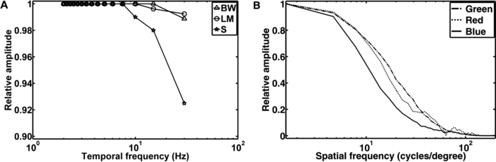 The measured frame delay caused by the LCoS electronic interface was 14 ms. The refresh rate of the projector (60 Hz) was verified. In a 120 min test, no variations in these measurements were observed over time. The minimum sMTF amplitude for the projector primaries occurs at ∼120 cycles/deg [Fig. 2b]. The blue spectrum exhibits the fastest decay in amplitude, whereas the red and green sMTFs are close together, with higher amplitudes. Optimal performance was achieved for the green primary with a spatial frequency of ∼17 cycles/deg at a relative amplitude of 0.5. At the same amplitude level, red has a spatial frequency of 14 cycles/deg and blue has a spatial frequency of 10.8 cycles/deg. 3.2.Digital Fundus ImagingFigures 3a and 3b show the measured camera sensitivity functions for the green and white spectra, respectively. The sensitivity functions reveal differences between the camera imagers and the test spectra. For the EMCCD and the CCD imager, both spectra have linear response functions. The CMOS camera clearly exhibits a nonlinear response. Its green sensitivity function has three different linear regions, with transitions at approximately 1 and 2.5 μW/cm2. In contrast, the white sensitivity function has only two linear regions, with a transition at 1.5 μW/cm2. Compared to the EMCCD and the CCD system, the absolute sensitivity of the CMOS system is markedly lower. Their relative differences to the CMOS imager are given in Fig. 4. At most response-signal levels, the relative sensitivity differences to the CMOS system are between 500 and 1000%. The EMCCD imager has higher differences in both the green and white spectra. For the green spectrum at a typical response level of 0.5, the CCD and EMCCD imagers are 423 and 565% more sensitive, respectively. Fig. 4Relative sensitivity differences of the EMCCD (circles) and CCD (asterisks) imager to the CMOS imager: (a) differences in the green sensitivities and (b) differences in the white sensitivities. 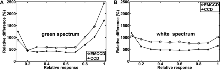 In this study, fundus imaging was performed using the EMCCD camera. Figure 5 shows fundus images and various stimulation patterns acquired with the EMCCD camera. Fig. 5Fundus of one volunteer and various stimulation patterns: (a) shows the fundus with MA (center of image). A circular SST flash with a black fixation point is shown in (b). Two different states of a checkerboard sequence are shown in (c) and (d). For selective modulation activity in the S-cone and the LM-cone pathway, we only used the SST flash stimulation.  3.3.EEG RecordingFigure 6 shows the measured VEPs and the GA responses (top) obtained in our previous study for S-cone simulation [Fig. 6a] and LM-cone [Fig. 6b] stimulation. The GAs from our previous study indicate a typical N1−P1 complex in the curve shapes of the S- and LM-cone responses. The mean peak-to-peak amplitude of the LM-cone response was ∼13 μV, which is higher than that of the S-cone response at 9 μV. The N1 latency of the LM-cone response (90 ms) is markedly smaller than that of the S-cone response (111 ms). The P1 latency was 140 ms for the LM-cone response and 182 ms for the S-cone response. Fig. 6Measured VEPs (V1–V6) and GA responses from our previous study20. (a) S-cone responses and (b) LM-cone responses are plotted. N1 and P1 latencies are indicated by the left and right vertical lines, respectively. All responses are from electrode Oz. 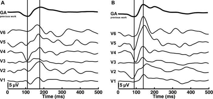 All volunteers in the present study showed high LM-cone peak-to-peak amplitudes (mean = 15 μV) with very good agreement in the N1 (mean = 89 ms) and P1 (mean = 143 ms) latencies. In the S-cone responses, smaller peak-to-peak amplitudes (mean = 9 μV) and higher N1 (mean = 113 ms) and P1 (mean = 170 ms) latencies were measured. The S-cone response of volunteer V3 was markedly smaller with a broad first positive wave. For a complete comparison with the GA responses, the slopes of the N1−P1 complex were also computed. Figure 7 shows the positions of four parameters (N1 latency, P1 latency, slope, peak-to-peak amplitude) for both responses of the volunteers in box plots of the GA responses obtained from our previous study. Almost all the N1 and P1 values for both silent substitution conditions are located in the box near the GA median. In the plot of the slope, two values for the S-cone response and three values for the LM-cone response lie within 1.5 times of the lower interquartile range. Apart from two LM-cone responses and one S-cone response, all peak-to-peak amplitudes are located below the box median. Five of the 12 responses lie within the lower interquartile range. One S-cone amplitude is markedly smaller than the others, lying below the bottom of the whiskers. Fig. 7Volunteers’ VEP parameters: (a) N1 latency, (b) P1 latency, (c) slope, and (d) peak-to-peak amplitude compared with the distribution of the GA responses from our previous study20. The GA box plots show (left) the S-cone response and (right) the LM-cone response. “+” symbols indicate the parameter positions of the measured VEPs (for better visualization, “+” symbols that overlap are plotted horizontally).  Figure 8 shows the VEPs of papilla (PA) versus those for central stimulation within the macula (MA) for volunteer V5. No response signals were measured after S- and LM-cone stimulations at the PA. In contrast, the central stimulation produces an S-cone VEP of ∼11 μV. For LM-cone modulation, the same position and area produces a VEP of ∼25 μV. 4.DiscussionTo the best of our knowledge, this paper presents the first optoelectrophysiological application to human volunteers that is suitable for modulating the S- and LM-cone pathways based on the fundus-controlled SST method. The new stimulation setup offers the possibility of simultaneously imaging the retina and electrophysiological investigating the retina morphologies of individuals. In recent years, the combination of retinal imaging, functional measurement, and stimulation techniques has become an important multidisciplinary field of research. In this context, Packer.29 and Pacer and Dacey30 developed one of the first devices for imaging retinal stimuli, combining a biological research microscope with a digital micromirror device (DMD) stimulator for projecting spatial patterns on the primate retina. Poloscheck. used a confocal scanning laser ophthalmoscope in combination with multifocal ERG recordings on human volunteers. One limitation of this approach was the typical stimulus generation by a 514-nm laser source, which is not appropriate for SST stimulation paradigms.31 Several research groups are currently focusing on applications of functional ultrahigh-resolution OCT (fUHROCT). 32, 33, 34, 35 An important study in this field was carried out by Bizheva., who observed local variations in the reflectivity of retina tissue caused by light stimulation. To investigate these functional correlations, they combined OCT with synchronous ERG recordings.32 All current fUHROCT devices are limited with respect to stimulus generation. To date, only bright, noncolored, visible-light stimuli have been used to activate the retina. Riva. combined laser doppler flowmetry with unstructured stimuli generated by red and green LEDs. They used different color ratios and a SST paradigm to determine the response of human optic nerve head blood flow.36 A review of other different optophysiological studies that explored the changes in hemodynamics and oxygenation in the retina and optic nerve in response to different stimuli is also given by Riva.37 In the present work, we designed a digital color LCoS projection stimulator suitable for fundus-controlled SST stimulation in humans. Our EEG measurements aimed for the investigation of selective S- and LM-cone responses without rod intrusion. Therefore, we studied light-adapted volunteers and employed an ambient-room luminance of 95 cd/m2. In combination with maximally dilated volunteer pupils, this caused a photopic retinal illuminance of ∼3.7 log phot td. Rod saturation is achieved at 2.7 log phot td.38 That is why their contributions in the response signals should be prevented. Figure 6 shows the measured S- and LM-cone VEPs, and compares them to the GA data from our previous study. Very good latency matches with the GA after combined stimulation are obtained for all volunteers. Compared to the LM-cone response, the VEP latencies after S-cone stimulation are typically higher, which is consistent with the findings of other researchers. 26, 39 Of the two stimulations, the LM-cone response produces higher amplitudes. Porciatti and Sartucci also found higher amplitudes for LM-cone responses after onset VEP examinations.26 Figure 7 presents the accurate positions of all computed parameters for both responses in box plots of the GA. The latency parameters for both stimulations are located near the median, confirming the assumption of a strong correlation with the GAs. The peak-to-peak amplitudes tend to be slightly smaller than those obtained in our previous study, possibly because of the smaller target area on the retina. Other researchers have observed a similar relationship between VEP amplitudes and stimulation area. 40, 41 The target areas in the present study are ∼53% smaller than those used in our previous study, due to the optical setup used in this study for imaging the 3LCoS panels into the fundus camera. Using a modified setup [especially with respect to lenses L2 and L3 (Fig. 1)], it should be possible to address a fundus area of 45 deg in a single image. On the basis of the characteristics of the measured parameters, the ability to produce stimuli to access both the S- and LM-cone pathways could be confirmed. To estimate the influence of stray light and the geometric accuracy of the optical imaging, we performed papillary stimulation and compared it to central stimulation (Fig. 8). Under ideal conditions, no VEP should be detectable. Research groups in the field of scotoma detection and microperimetry agree with this hypothesis. 42, 43 These groups were also unable to detect PA response signals for stimulation spot sizes similar to those used in the present study. Meyer. found that the PA topography affects stray light generation at larger spot sizes and luminances. Consequently, responses from the nasal fundus are expected.43 However, no VEP response was observed for either SST stimulation at the PA. The temporal and spatial performance of the new stimulator was evaluated using modulation transfer functions. The temporal properties of a stimulus are known to affect VEPs. Several researchers have discovered fundamental differences in physiologic responses depending on the time characteristics of the stimulation techniques used, such as LCD, DMD, LED, and cathode ray tube. 44, 45, 46 The most critical part of flash sequences is the electro-optical response behavior, which influences the effective stimulation contrast and the cone contrast for SST application. The tMTFs shown in Fig. 2a have a minimal contrast loss of 7% for the S-cone sequence at the highest stimulation frequency (30 Hz). An increase in latencies with a reduced contrast, as described by Jakobsson and Johansson,47 Porciatti and Sartucci,26 and Rabin.,48 could not be confirmed for this contrast loss. Nearly perfectly flat tMTFs could be achieved only with the black−white flicker and LM-cone flicker. In contrast, Packer. realized a contrast loss of 60% at 31.5 Hz with the DMD technique.29 The sMTFs for the projector primaries plotted in Fig. 2b have maximum spatial frequencies of ∼120 cycles/deg. High luminance contrast stimuli could be generated at a typical sMTF amplitude of 0.5. Under this condition, spatial frequencies of 10.8 cycles/deg (blue primary), 14 cycles/deg (red primary), and 17 cycles/deg (green primary) can be applied. This is equivalent to a smallest projectable element on the fundus in the range of 2.7–1.8 arcmin. Thus, the new stimulator can be used for all paradigms without restriction for the ISCEV standard for clinical VEPs4 (smallest element size: 15 arcmin). Because visual responses become faster and their amplitude increases with increasing stimulus intensity, 49, 50 we adjusted the light output of the LCoS projector. The white-spectrum radiant flux of the previous LCD stimulator system was used as a basis for the computation, enabling us to compare the EEG data from both studies. The pupil area for the field luminance of the LCD system could not be measured, but it was estimated using the expression given by Reeves.22 Other formulas for estimating the pupil are given in the literature, 51, 52 but they all have low modulation accuracies. A slight adjustment error is expected due to this estimation error. The smaller peak-to-peak amplitudes could be caused by the adjustment error in addition to the smaller stimulation area. The light level after adjusting the LCoS projector (radiant flux = 0.63 mW) was significantly lower than that of conventional fundus cameras. Because the image quality of digital cameras depends on the light level, we tested the sensitivities of three systems under different spectral conditions. In addition to the white spectrum, we analyzed the green spectrum separately to assess the ability of the cameras to produce high-contrast images at the optimal fundus orientation. Conventional fundus cameras employ special optical filters in the green light range to generate high-contrast images. Figures 3 and 4 reveal distinct differences between the CMOS, CCD, and EMCCD devices. Researchers from various scientific fields have performed similar tests and found that CMOS imagers tend to have higher noise levels and lower sensitivities than do CCD imagers. 53, 54 However, the image quality of the EMCCD camera used in this study is inferior to that of conventional fundus cameras due to the low light level. Fig. 3Sensitivity functions of the CMOS (triangles), EMCCD (circles), and CCD (asterisks) imager for (a) the green spectrum and (b) the white spectrum of the projector.  The presented results demonstrate that optoelectrophysiological stimulation and measurement of the human retina is possible using the new fundus-controlled projection stimulator. SST stimuli paradigms for accessing the S- and LM-cone pathways can be simultaneously combined with morphological fundus data. The functional integrity of retinal areas can be examined under direct fundus control. To further validate this optoelectrophysiological methodology, it is necessary to perform studies with several patients diagnosed with glaucoma or macular degeneration. Therefore, the next steps will be to increase the target area of the stimuli and to enhance the fundus image quality. AcknowledgmentsThe authors thank Sven Krüger (HOLOEYE Photonics AG) and Volker Gäbler (High Technology Services) for the help with the projector. This research was supported by the German Federal Ministry of Education and Research (Grant No. 03IP605). ReferencesG. E. Holder,
“Electrophysiological assessment of optic nerve disease,”
Eye, 18 1133
–1143
(2004). https://doi.org/10.1038/sj.eye.6701573 Google Scholar
A. B. Renner, U. Kellner, H. Tillack, H. Kraus,
“Recording of both VEP and multifocal ERG for evaluation of unexplained visual loss—Electrophysiology in unexplained visual loss,”
Doc. Ophthalmo., 111 149
–157
(2005). https://doi.org/10.1007/s10633-005-5362-4 Google Scholar
G. E. Holder, M. G. Brigell, M. Hawlina, T. Meigen, X. Vaegan, and
M. Bach,
“ISCEV standard for clinical pattern electroretinography–2007 update,”
Doc. Ophthalmol., 114 111
–116
(2007). https://doi.org/10.1007/s10633-007-9053-1 Google Scholar
J. V. Odom, M. Bach, M. Brigell, G. E. Holder, D. L. McCulloch, A. P. Tormene,
“ISCEV standard for clinical visual evoked potentials (2009 update),”
Doc. Ophthalmol., 120 111
–119
(2009). https://doi.org/10.1007/s10633-009-9195-4 Google Scholar
O. Estevez and
H. Spekreijse,
“The “silent substitution” method in visual research,”
Vis. Res., 22 681
–691
(1982). https://doi.org/10.1016/0042-6989(82)90104-3 Google Scholar
V. C. Smith, J. Pokorny, M. Davis, and
T. Yeh,
“Mechanisms subserving temporal-modulation sensitivity in silent-cone substitution,”
J. Opt. Soc. Am. A, 12 241
–249
(1995). https://doi.org/10.1364/JOSAA.12.000241 Google Scholar
B. B. Lee, P. R. Martin, and
A. Valberg,
“Sensitivity of macaque retinal ganglion-cells to chromatic and luminance flicker,”
J. Physiol.-Lond., 414 223
–243
(1989). Google Scholar
S. Engel, X. M. Zhang, and
B. Wandell,
“Colour tuning in human visual cortex measured with functional magnetic resonance imaging,”
Nature, 388 68
–71
(1997). https://doi.org/10.1038/40398 Google Scholar
A. Chaparro, C. F. Stromeyer, G. Chen, and
R. E. Kronauer,
“Human cones appear to adapt at low-light levels—measurements on the red-green detection mechanism,”
Vis. Res., 35 3103
–3118
(1995). https://doi.org/10.1016/0042-6989(95)00069-C Google Scholar
J. Kremers, T. Usui, H. P. N. Scholl, and
L. T. Sharpe,
“Cone signal contributions to electrograms in dichromats and trichromats,”
Invest. Ophthalmol. Vis. Sci., 40 920
–930
(1999). Google Scholar
F. J. Rucker and
P. B. Kruger,
“Accommodation responses to stimuli in cone contrast space,”
Vision Research, 44 2931
–2944
(2004). https://doi.org/10.1016/j.visres.2004.07.005 Google Scholar
A. Stockman and
L. T. Sharpe,
“The spectral sensitivities of the middle- and long-wavelength-sensitive cones derived from measurements in observers of known genotype,”
Vis. Res., 40 1711
–1737
(2000). https://doi.org/10.1016/S0042-6989(00)00021-3 Google Scholar
A. F. Fercher, C. K. Hitzenberger, W. Drexler, G. Kamp, and
H. Sattmann,
“In-vivo optical coherence tomography,”
Am. J. Ophthalmol., 116 113
–115
(1993). Google Scholar
R. A. Leitgeb, W. Drexler, A. Unterhuber, B. Hermann, T. Bajraszewski, T. Le, A. Stingl, and
A. F. Fercher,
“Ultrahigh resolution Fourier domain optical coherence tomography,”
Opt. Express, 12 2156
–2165
(2004). https://doi.org/10.1364/OPEX.12.002156 Google Scholar
M. Wojtkowski, R. Leitgeb, A. Kowalczyk, T. Bajraszewski, and
A. F. Fercher,
“In vivo human retinal imaging by Fourier domain optical coherence tomography,”
J. Biomed. Opt., 7 457
–463
(2002). https://doi.org/10.1117/1.1482379 Google Scholar
Y. M. Wang, B. A. Bower, J. A. Izatt, O. Tan, and
D. Huang,
“Retinal blood flow measurement by circumpapillary Fourier domain Doppler optical coherence tomography,”
J. Biomed. Opt., 13 064003
(2008). https://doi.org/10.1117/1.2998480 Google Scholar
M. Miura, M. Yamanari, T. Iwasaki, A. E. Elsner, S. Makita, T. Yatagai, and
Y. Yasuno,
“Imaging polarimetry in age-related macular degeneration,”
Invest. Ophthalmol. Vis. Sci., 49 2661
–2667
(2008). https://doi.org/10.1167/iovs.07-0501 Google Scholar
M. Yamanari, M. Miura, S. Makita, T. Yatagai, and
Y. Yasuno,
“Phase retardation measurement of retinal nerve fiber layer by polarization-sensitive spectral-domain optical coherence tomography and scanning laser polarimetry,”
J. Biomed. Opt., 13 199
–204
(2008). https://doi.org/10.1117/1.2841024 Google Scholar
X. R. Huang and
R. W. Knighton,
“Linear birefringence of the retinal nerve fiber layer measured in vitro with a multispectral imaging micropolarimeter,”
J. Biomed. Opt., 7 199
–204
(2002). https://doi.org/10.1117/1.1463050 Google Scholar
P. Bessler, S. Klee, U. Kellner, and
J. Haueisen,
“Silent substitution stimulation of S-cone pathway and L- and M-cone pathway in glaucoma,”
Invest. Ophthalmol. Vis. Sci., 51 319
–326
(2010). https://doi.org/10.1167/iovs.09-3467 Google Scholar
H. Gross, M. Totzeck, and
W. Singer, Handbook of Optical Systems, Wiley-VCH, Weinheim
(2005). Google Scholar
P. Reeves,
“The response of the average pupil to various intensities of light,”
J. Opt. Soc. Am., 4 35
–43
(1920). https://doi.org/10.1364/JOSA.4.000035 Google Scholar
D. Atchison and
G. Smith, Optics of the Human Eye, Butterworth Heinemann, Edinburgh2000). Google Scholar
R. W. G. Hunt,
“Revised color-appearance model for related and unrelated colors,”
Color Res. Appl., 16 146
–165
(1991). https://doi.org/10.1002/col.5080160306 Google Scholar
R. W. G. Hunt, C. J. Li, and
M. R. Luo,
“Dynamic cone response functions for models of colour appearance,”
Color Res. Appl., 28 82
–88
(2003). https://doi.org/10.1002/col.10128 Google Scholar
V. Porciatti and
F. Sartucci,
“Normative data for onset VEPs to red-green and blue-yellow chromatic contrast,”
Clin. Neurophysiol., 110 772
–781
(1999). https://doi.org/10.1016/S1388-2457(99)00007-3 Google Scholar
A. Stockman and
L. T. Sharpe,
“Cone spectral sensitivities and color matching,”
52
–87 Cambridge University Press, Cambridge
(1999). Google Scholar
G. Sporckmann,
“Signalerfassung, Signalverarbeitung und Mustererkennung bei visuell evozierten Potentialen zur verbesserten objektiven Diagnostik der menschlichen Sehleistung,”
(1996) Google Scholar
O. Packer, L. C. Diller, J. Verweij, B. B. Lee, J. Pokorny, D. R. Williams, D. M. Dacey, and
D. H. Brainard,
“Characterization and use of a digital light projector for vision research,”
Vis. Res., 41 427
–439
(2001). https://doi.org/10.1016/S0042-6989(00)00271-6 Google Scholar
O. S. Packer and
D. M. Dacey,
“Synergistic center-surround receptive. field model of monkey H1 horizontal cells,”
J. Vis., 5 1038
–1054
(2005). https://doi.org/10.1167/5.11.9 Google Scholar
C. M. Poloschek, V. Rupp, H. Krastel, and
F. G. Holz,
“Multifocal ERG recording with simultaneous fundus monitoring using a confocal scanning laser ophthalmoscope,”
Eye, 17 159
–166
(2003). https://doi.org/10.1038/sj.eye.6700294 Google Scholar
K. Bizheva, R. Pflug, B. Hermann, B. Povazay, H. Sattmann, P. Qiu, E. Anger, H. Reitsamer, S. Popov, J. R. Taylor, A. Unterhuber, P. Ahnelt, and
W. Drexler,
“Optophysiology: Depth-resolved probing of retinal physiology with functional ultrahigh-resolution optical coherence tomography,”
Proc. Natl. Acad. Sci. USA, 103 5066
–5071
(2006). https://doi.org/10.1073/pnas.0506997103 Google Scholar
W. Drexler,
“Cellular and functional optical coherence tomography of the human retina—the Cogan lecture,”
Invest. Ophthalmol. Vis. Sci., 48 5340
–5351
(2007). https://doi.org/10.1167/iovs.07-0895 Google Scholar
V. J. Srinivasan, Y. Chen, J. S. Duker, and
J. G. Fujimoto,
“In vivo functional imaging of intrinsic scattering changes in the human retina with high-speed ultrahigh resolution OCT,”
Opt. Express, 17 3861
–3877
(2009). https://doi.org/10.1364/OE.17.003861 Google Scholar
L. Kagemann, G. Wollstein, M. Wojtkowski, H. Ishikawa, K. A. Townsend, M. L. Gabriele, V. J. Srinivasan, J. G. Fujimoto, and
J. S. Schuman,
“Spectral oximetry assessed with high-speed ultra-high-resolution optical coherence tomography,”
J. Biomed. Opt., 12 041212
(2007). https://doi.org/10.1117/1.2772655 Google Scholar
C. E. Riva, B. Falsini, and
E. Logean,
“Flicker-evoked responses of human optic nerve head blood flow: Luminance versus chromatic modulation,”
Invest. Ophthalmol. Vis. Sci., 42 756
–762
(2001). Google Scholar
C. E. Riva, E. Logean, and
B. Falsini,
“Visually evoked hemodynamical response and assessment of neurovascular coupling in the optic nerve and retina,”
Prog. Retinal Eye Res., 24 183
–215
(2005). https://doi.org/10.1016/j.preteyeres.2004.07.002 Google Scholar
A. Stockman and
L. T. Sharpe,
“Into the twilight zone: the complexities of mesopic vision and luminous efficiency,”
Ophthal. Physiol. Opt., 26 225
–239
(2006). https://doi.org/10.1111/j.1475-1313.2006.00325.x Google Scholar
D. J. McKeefry, N. R. Parry, and
I. J. Murray,
“Simple reaction times in color space: the influence of chromaticity, contrast, and cone opponency,”
Invest. Ophthalmol. Vis. Sci., 44 2267
–2276
(2003). https://doi.org/10.1167/iovs.02-0772 Google Scholar
H. A. Baseler, E. E. Sutter, S. A. Klein, and
T. Carney,
“The topography of visual evoked response properties across the visual field,”
Electroencephalogr. Clin. Neurophysiol., 90 65
–81
(1994). https://doi.org/10.1016/0013-4694(94)90114-7 Google Scholar
C. Yiannikas and
J. C. Walsh,
“The variation of the pattern shift visual evoked-response with the size of the stimulus field,”
Electroencephalog. Clin. Neurophysiol., 55 427
–435
(1983). https://doi.org/10.1016/0013-4694(83)90131-1 Google Scholar
T. Bek and
H. Lundandersen,
“The influence of stimulus size on perimetric detection of small scotomata,”
Graefes Arch. Clin. Exp. Ophthalmol., 227 531
–534
(1989). https://doi.org/10.1007/BF02169446 Google Scholar
J. H. Meyer, M. Guhlmann, and
J. Funk,
“Blind spot size depends on the optic disc topography: A study using SLO controlled scotometry and the Heidelberg retina tomograph,”
Br. J. Ophthalmol., 81 355
–359
(1997). https://doi.org/10.1136/bjo.81.5.355 Google Scholar
C. Kaltwasser, F. K. Horn, J. Kremers, and
A. Juenemann,
“A comparison of the suitability of cathode ray tube (CRT) and liquid crystal display (LCD) monitors as visual stimulators in mfERG diagnostics,”
Doc. Ophthalmol., 118 179
–189
(2008). Google Scholar
D. Keating, S. Parks, D. C. Smith, and
A. L. Evans,
“Using an LED stimulator to investigate the effect of stimulation frequency on the multifocal ERG,”
Invest. Ophthalmol. Vis. Sci., 44 32
(2003). https://doi.org/10.1167/iovs.01-1171 Google Scholar
T. J. Gawne and
J. M. Woods,
“Video-rate and continuous visual stimuli do not produce equivalent response timings in visual cortical neurons,”
Vis. Neurosci., 20 495
–500
(2003). https://doi.org/10.1017/S0952523803205034 Google Scholar
P. Jakobsson and
B. Johansson,
“The effect of spatial-frequency and contrast on the latency in the visual evoked-potential,”
Doc. Ophthalmol., 79 187
–194
(1992). https://doi.org/10.1007/BF00156577 Google Scholar
J. Rabin, E. Switkes, M. Crognale, M. E. Schneck, and
A. J. Adams,
“Visual evoked potentials in three-dimensional color space: correlates of spatio-chromatic processing,”
Vis. Res., 34 2657
–2671
(1994). https://doi.org/10.1016/0042-6989(94)90222-4 Google Scholar
T. Kammer, L. Lehr, and
K. Kirschfeld,
“Cortical visual processing is temporally dispersed by luminance in human subjects,”
Neurosci. Lett., 263 133
–136
(1999). https://doi.org/10.1016/S0304-3940(99)00137-8 Google Scholar
B. Link, S. Ruhl, A. Peters, A. Junemann, and
F. K. Horn,
“Pattern reversal ERG and VEP—comparison of stimulation by LED, monitor and a Maxwellian-view system,”
Doc. Ophthalmol., 112 1
–11
(2006). https://doi.org/10.1007/s10633-005-5865-z Google Scholar
P. Moon and
D. E. Spencer,
“Visual Data Applied to Lighting Design,”
J. Opt. Soc. Am., 34 605
–614
(1944). https://doi.org/10.1364/JOSA.34.000605 Google Scholar
S. G. Degroot and
J. W. Gebhard,
“Pupil Size As Determined by Adapting Luminance,”
J. Opt. Soc. Am., 42 492
–495
(1952). https://doi.org/10.1364/JOSA.42.000492 Google Scholar
J. Laitinen, J. Saviaro, and
H. Ailisto,
“Evaluation of solid-state camera systems in varying illumination conditions,”
Opt. Eng., 40 896
–901
(2001). https://doi.org/10.1117/1.1365937 Google Scholar
J. P. Golden and
F. S. Ligler,
“A comparison of imaging methods for use in an array biosensor,”
Biosens. Bioelectron., 17 719
–725
(2002). https://doi.org/10.1016/S0956-5663(02)00060-X Google Scholar
|


