|
|
1.IntroductionFluorescence spectroscopy has been widely explored in the field of pre-clinical and clinical cancer research over the past two decades.1–10 Intrinsic tissue fluorescence spectra reflect both the identity and concentration of endogenous tissue fluorophores. Common tissue fluorophores provide information about structural properties of the tissue (through collagen or elastin fluorescence),1,11 metabolic activity of the tissue [through important biological co-factors, reduced nicotinamide adenine dinucleotide (NADH) and flavin adenine dinucleotide (FAD)]12,13 or tissue micro-environmental changes (through porphyrin, tryptophan, or vitamin A fluorescence).4,6,14–16 Exogenous fluorophores/contrast agents such as 2-[N-(7-nitrobenz-2-oxa-1,3-diazol-4-yl)amino]-2-deoxyglucose or (2-NBDG), which is an optical analog to fluoro deoxy glucose, proflavine, which is a micro anatomical stain, and perfusion dyes, such as fluorescein and indocyanin green (ICG), have also been used as sources of contrast in tissue fluorescence studies.14,17–21 In addition, fluorescence spectroscopy for determining drug concentrations may provide a rapid and effective way for monitoring therapeutic efficacy by quantifying drug delivery/uptake in tumors.17–19 It is well known that the fluorescence measured from biological tissues is significantly distorted by tissue absorption and scattering. Knowledge of true fluorescence disentangled from the effects of absorption and scattering can improve contrast.10,22,23 For example, studies by Sterenborg et al.10 showed that there were no significant differences in directly measured auto fluorescence between normal skin and non-melanoma skin cancer, while Rajaram et al.22 drew the opposite conclusion after they corrected the measured tissue fluorescence for the distorting effects of absorption and scattering. Another study by Fawzy et al.23 also showed that the diagnostic content of fluorescence spectra measured from the lung was masked by tissue absorption and scattering. Georgakoudi et al.24 demonstrated decreased collagen and increased NADH contributions in both dysplastic cervical and Barrett’s esophagus tissues (relative to normal sites), via the use of intrinsic fluorescence extracted from turbid tissue fluorescence. These examples along with others9,11,25,26 demonstrate that extraction of intrinsic fluorescence not only enhances contrast but it also aids in the interpretation of the metabolic, structural, and biochemical information contained in the tissue fluorescence. Palmer et al.18 have successfully conducted a study to quantitatively monitor drug delivery and accumulation based on spectra of turbidity-free drug fluorescence (intrinsic fluorescence of Doxorubicin) that was detected noninvasively and in vivo in a murine xenograft model. By correcting for tissue turbidity, the authors were able to quantify fluorophore concentration/accumulation in vivo and show that turbidity-free fluorescence spectroscopy could provide critical insight into in vivo pharmacokinetics of the drug inside rodent tumors. A number of reports have been published to disentangle the effects of absorption and scattering from the measured fluorescence spectrum to recover the intrinsic fluorescence spectra.27–35 These studies have used theoretical methods based on physical models of light-tissue interactions, including analytical approaches based on diffusion theory32–35 as well as computational techniques such as Monte Carlo simulations of photon transport in turbid media29–31 or simple empirical approaches.27,28 The empirical approaches use simple ratios of intensities at specific wavelengths to obtain endpoints that correlate with the intrinsic fluorescence and will not be discussed further here. The discussion will focus on diffusion and Monte Carlo based approaches. Diffusion theory is an approximation to the radiative transport equation and describes photon transport in absorbing and scattering media. Thus it can correct the measured fluorescence spectrum based on the tissue absorption and scattering properties to extract the intrinsic fluorescence spectrum analytically. However, the diffusion approximation is only valid when the absorption coefficient of the medium is at least an order of magnitude lower than scattering and for sources and detectors that are separated from each other by distances much greater than the mean free path of diffusing photons in that medium [this typically corresponds to the red and near infrared spectral (NIR) regions].36 The Monte Carlo method is stochastic in nature and is not limited to the diffusion regime. It can therefore be used to model light transport over the entire UV-visible-NIR range. However, Monte Carlo simulations are computationally time-consuming and have historically not been very convenient to use as inverse models,37 which is the reason that it is mostly used in combination with other methods such as the diffusion approximation for intrinsic fluorescence extraction.29,31,38,39 Our group has developed an inverse Monte Carlo model40,41 that addresses the computational speed issues of conventional Monte Carlo modeling via a simple scaling technique. This model has been shown to be able to accurately correct for both the shape and overall intensity of fluorescence measured in a scattering and absorbing tissue phantom.41 The original study published by our group served to primarily demonstrate the methodology for extracting intrinsic fluorescence in turbid tissue mimicking phantoms and to test the impact of a wide range of absorption and scattering properties on recovery of the true fluorescence spectral shape and intensity of a single fluorophore at a fixed concentration that was embedded in the phantoms. This new publication builds on our original work toward the goal of measuring intrinsic and extrinsic fluorescence that reflects tissue bioenergetics. The first objective is to demonstrate the versatility of our Monte Carlo based model in tissue mimicking phantoms containing multiple fluorophores (over a wide range of fluorophore concentrations and wavelengths) in a background of absorbers and scatterers. The choices of fluorophores in the tissue mimicking phantoms were guided by both endogenous and exogenous fluorophores that specifically report on tissue metabolism. Three fluorophores—NADH, 2-NBDG and Tetra Methyl Rhodamine (TMR)—were considered. NADH [340-nm excitation maximum (exc.), 465-nm emission maximum (em.)] is an endpoint of cellular glycolysis and an indicator of tissue reduction-oxidation ratio when measured in combination with FAD;12,13,42 2-NBDG (470-nm exc.; 550-nm em.) is an optical analog to FDG and can report on glucose uptake;43 and TMR (557-nm exc.; 576-nm em.) can be used to probe mitochondrial trans-membrane potential and thus report on mitochondrial activity.44 The second objective is to demonstrate the capability of the model to quantify the uptake-kinetics of the intrinsic fluorescence of 2-NBDG as a function of dose and time in a pre-clinical model of breast cancer. 2.Materials and Methods2.1.Tissue PhantomsTissue-mimicking phantoms that had varying amounts of absorption, scattering, and fluorophore concentrations were prepared. Hemoglobin (H0267, Sigma-Aldrich Co., St. Louis, MO) was used as the non-fluorescent absorber and 1-μm monodisperse polystyrene spheres (1-μm diameter, Catalog No. 07310, Polysciences, Warrington, PA) was used as the scatterer in tissue-mimicking phantoms following the procedures described in detail previously.45,46 Mixing known volumes of stock hemoglobin (absorber) solution and microsphere suspensions in deionized (DI) water with stock fluorophore solution allowed accurate control of the final absorption, scattering, and fluorescence properties in each phantom. The absorption spectra of the stock and stock fluorophore solutions [measured using a spectrophotometer (Cary 300, Varian, Inc.)] were used to determine the final absorption of the phantom, while the values of the reduced scattering coefficients in the phantoms were calculated from the Mie theory for spherical particles using freely available software.47 Three distinct fluorophores were used in this study: Stilbene 3 (04200, Exciton, Dayton, Ohio) was used as an analog for NADH fluorescence,22,48 2-NBDG (N13195, Invitrogen, Carlsbad, CA), and Rhodamine B (R6626, Sigma-Aldrich Co., St. Louis, MO) was used to represent fluorescence of TMR as their spectra are very similar.49 The spectral range spanned by the fluorescence emission of these three fluorophores covers the three distinct absorption bands (soret, alpha, and beta bands) of the oxy hemoglobin () absorption spectrum. Since hemoglobin is the principal absorber in most human and animal tissues, these choices would also allow us to evaluate the effects of hemoglobin absorption on the detected fluorescence spectra. Figure 1 shows the emission spectra of these fluorophores (and NADH) along with the absorption spectrum of . Fig. 1(a) Normalized absorption spectrum (Soret band region, 380 to 430 nm) along with emission spectra of NADH (340-nm exc.) and Stilbene (350-nm exc.), which are similar to each other, although the NADH fluorescence maximum is slightly red-shifted and (b) normalized absorption spectrum (alpha-beta band region, 520 to 590 nm) with emission spectra of 2-NBDG (470-nm exc.) and Rhodamine B (545-nm exc.).  Six different sets of tissue phantoms containing one or more fluorophores were prepared. Table 1 summarizes the optical properties and fluorophore concentrations in the phantoms and the corresponding measurement parameters. The value of the optical absorption and scattering properties used here were based on our previous estimates of optical properties of murine tumors (, , averaged between 350 to 650 nm).50 Each phantom set contained two subsets: these two subsets either had two different absorption levels with same scattering, or two levels of scattering with the same absorption level. Each subset contained a phantom with increasing fluorophore concentrations through sequential additions of small volumes of fluorophore stock solution. Each phantom was identified through a code made up of an alphabet and two digits (A11 through F27). The alphabet denotes the main phantom set, the first digit represents the optical absorption ()/scattering () level and last digit corresponds to the fluorophore concentration level in that subset (see Table 1). For each phantom set, the range of fluorophore concentrations in the two phantom subsets were identical; for example, both phantoms in the pairs A11 & A21, A12 & A22, A31 & A32, and A14 & A24 had the same fluorophore concentration, while phantoms A11 through A14 spanned a range of four different fluorophore concentrations. Phantom sets E and F contained two fluorophores, and therefore the concentrations of both fluorophores were increased simultaneously. Fluorophore solutions (containing only the fluorophore in water without any absorber and scatterer) with the same fluorophore concentrations as in the phantoms across each set were measured to get the measured intrinsic fluorescence free of absorption and scattering using the same illumination and collection geometry and instrument. These are referred to as the non-turbid fluorophore solution. Table 1Absorption, scattering, and fluorescence properties and measurement parameters within each phantom set. The listed optical properties represent the average value between 350 and 650 nm (* means excitation wavelength).
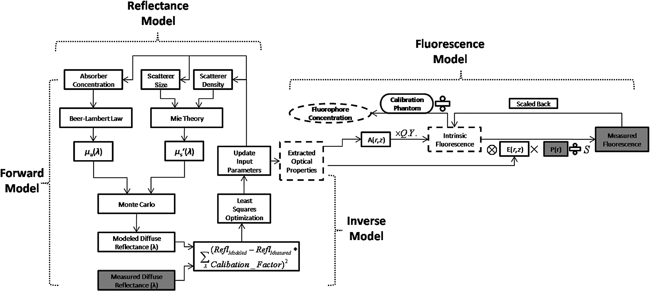
2.2.In Vivo Murine Breast Cancer ModelAll in vivo experiments were conducted according to a protocol approved by the Duke University Institutional Animal Care and Use Committee. Six- to eight-week-old female athymic nude mice (nu/nu, NCI, Frederic, MD) weighing 25 to 30 g were used in these studies. Animals were housed in an onsite housing facility with ad libitum access to food and water and standard 12-h light/dark cycles. All animal experiments were conducted during the day, and mice were fasted for six hours prior to optical measurements. Fasting ensured that glucose in the body did not compete with 2-NBDG uptake and good signal contrast from the tumor compared to normal tissue. A 4T1 murine breast cancer cell line was used to grow flank tumors in these mice. The 4T1 cells were transduced with retroviral siRNA to constitutively express the red fluorescence protein (RFP), DsRed. Each mouse received a subcutaneous injection of 750,000 cells in an injection volume of 100 μl. Flank tumors were monitored every other day and allowed to grow to a volume [] of . A total of eight tumor-bearing animals were divided into three groups and each group received 2, 4 or 6 mM of 2-NBDG (two animals in 2 mM group, three in 4 mM group, and three in 6 mM group). A volume of 100 μl of 2-NBDG was injected systemically through the tail-vein of the mouse. 2.3.Optical MeasurementsA commercial fluorometer (SkinSkan, J.Y. Horiba, Edison, NJ) coupled to a fiber-optic bundle was used for all the reflectance and fluorescence measurements. The instrument consists of a 150-W xenon lamp as the light source, dual excitation, and emission-grating monochromators, each having a fixed spectral band pass of 5 nm and an extended red photomultiplier tube (PMT) as the detector. Diffuse reflectance measurements were collected by synchronously scanning the excitation and emission monochromators across the wavelength range of interest. Fluorescence measurements were collected by fixing the source monochromator to provide the required excitation wavelength while scanning the detection monochromator over the desired spectral range (Table 1 shows both reflectance and fluorescence wavelengths for phantom measurement). The instrument coupled the excitation to the sample and collected detected light from the sample via a bifurcated fiber-optic probe bundle. The common (sample) end of the fiber probe had 59 individual fibers (with illumination and collection fibers having numerical apertures of 0.125 and 0.12, respectively) with each individual fiber having a core/cladding diameter of . The arrangement of the fibers within the optical probe is described in an earlier study.25 Using forward Monte Carlo simulations as described in previous studies,51,52 this probe was computed to have a sensing depth (defined as the maximum depth that 90% of diffusely reflected photons ever penetrated) of 1 to 3 mm for the range of optical properties listed in Table 1. Single time repeated reflectance and fluorescence spectra were measured from both the phantom and animal models. Reflectance and fluorescence scans from the phantoms were obtained by placing the optical probe just beneath the surface of the liquid with the phantom being stirred using magnetic stirrers the entire time to prevent polystyrene spheres from settling. The optical measurement protocol for the animal tumors was as follows. The animals were anesthetized via Isoflurane breathing (1.5% Isoflurane gas mixed with oxygen) throughout the course of the optical measurements. Reflectance and fluorescence spectra were acquired sequentially from the tumor for 80 minutes (with a cycle time of 100 s) by gently pushing the probe to make contact with the tumor and stabilizing it using a clamp during the measurements. Reflectance spectra were acquired from 450 to 650 nm, and fluorescence emission spectra were acquired from 510 to 600 nm using excitation at 490 nm. An excitation wavelength of 490 nm was used rather than 470 nm as in 2-NBDG phantom studies to minimize endogenous FAD contribution. Prior to 2-NBDG injection, baseline reflectance and fluorescence spectra were measured from the tumor site. In both phantom and animal studies, the integration time of the photodetector was 0.1 s per wavelength for reflectance scans and 3 s per wavelength for fluorescence scans. All the measurements for both phantom and animal studies were acquired in a dark room. Optical spectroscopy measurements on both the phantoms and animal models were conducted after adequate time was allowed for system warm up () and under same probe-bending conditions to minimize their impact on the systematic errors reported in an earlier study.53 Overall system throughput variation on different days was assessed by measuring the reflectance from a Spectralon reflectance standard SRS-99 (Labsphere Inc., North Sutton, NH) and the fluorescence from a Rhodamine standard slide (590-nm exc., 610 to 680-nm em.) on three different days. The coefficient of variance of the collected spectra (calculated as where , , and are the reflectance or fluorescence spectra measured on three different days, and is the wavelength term) varied by less than 2% for both reflectance and fluorescence across the entire spectral range. The wavelength-dependent response of the monochromators, fiber bundle, and PMT on the measured fluorescence spectra was corrected by multiplying the spectra with a calibration factor that was obtained by dividing the theoretical lamp spectrum of a tungsten calibration lamp standard (Optronic Laboratories Inc., Orlando, FL) provided by the manufacturer to the instrument output of the lamp.2.4.Inverse Monte Carlo Models for Reflectance and FluorescenceThe measured reflectance and system response calibrated fluorescence spectra for both phantom and pre-clinical studies were input into a series of scalable inverse Monte Carlo models. The scalable inverse Monte Carlo models for extracting optical properties and intrinsic fluorescence have previously been described and validated experimentally on optical tissue phantoms containing a single fluorophore.41 In order to correct the measured fluorescence spectrum, it is necessary to know the optical absorption and scattering properties of the medium, which are first extracted from the measured diffuse reflectance spectrum using the inverse Monte Carlo reflectance model.40 These extracted optical properties are then used by the inverse Monte Carlo fluorescence model to remove the distortions in the measured fluorescence spectrum to provide the intrinsic fluorescence.40,41 Figure 2 shows the inputs and outputs to the inverse MC reflectance and fluorescence models, which themselves are further deconstructed in Fig. 3. Figure 3 is a detailed flowchart of the model itself, with inputs in gray boxes and outputs in boxes with a dashed outline (“Measured Fluorescence” in the gray box means system response calibrated fluorescence). The reflectance model40 consists of a forward and an inverse component. In the forward component, the wavelength-dependent absorption coefficients of the medium are calculated from the concentration of each absorber that is present in the medium and their corresponding wavelength-dependent extinction coefficients, while the wavelength-dependent reduced-scattering coefficients are calculated from scatterer size, density, and the refractive index of the scatterer and surrounding medium using Mie theory for spherical particles. The absorption and scattering coefficients are then used by the reflectance model to rapidly compute a modeled diffuse reflectance spectrum. The inverse component works by adaptively fitting the modeled diffuse reflectance to the measured tissue diffuse reflectance till the sum of squares error between the modeled and measured diffuse reflectance is minimized. A simulated and measured “reference” phantom with known optical properties is used to generate the calibration factor to put the experimental and simulated reflectance data on the same scale. The phantom reflectance spectra were calibrated to a reference phantom spectrum from the same phantom data set (phantom A14, B22, C21, D22, E12, F13 in each set) based on a previously used protocol,45 i.e., the reference phantom should yield the lowest error when used to extract optical properties from the remaining phantoms in the same phantom data set. The reflectance spectra from the animals were calibrated to phantom F13 based on the same criteria. The concentrations of absorber, scatterer size, and density that match the measured reflectance are used to calculate the extracted optical properties. The fluorescence model can be described by the following equation: where is the fluorescence quantum yield, is the fluorophore concentration, is the extinction coefficient of the fluorophore at the excitation wavelength, is the absorption coefficient of the fluorophore at the excitation wavelength, and is the total absorption coefficient of all absorbers in the medium at the excitation wavelength. The term describes the probability of an absorbed photon being absorbed by the fluorophore rather than other non-fluorescent absorbers. is the spectral probability distribution of the generated fluorescence as a function of the emission wavelength, so gives the probability that a generated fluorescence photon will be emitted at the emission wavelength . is the absorbed excitation energy density grid in a cylindrical coordinate generated using forward Monte Carlo simulations based on the optical properties at the excitation wavelength extracted from the inverse Monte Carlo reflectance model. So gives the generated fluorescence energy density at each grid element as a function of emission wavelength, which will also be the intrinsic fluorescence. The generated intrinsic fluorescence will be reabsorbed and scattered so only part of the energy will eventually exit the surface of the tissue. defines the possibility that a fluorescence photon originating at the coordinate will exit the surface of the medium at coordinate , which is also based on forward Monte Carlo simulations using the extracted optical properties at the emission wavelength. So, gives the fluorescence energy density that will escape the surface of the medium. The overall fluorescence energy exiting the surface of the medium will be a discrete sum up of all the grids over (grid surface area) and (grid depth dimension). The exiting fluorescence energy will only be partly picked up by the collection fibers of the probe, and this is accounted for by the factor.40 is a scaling factor to put the MC simulated result and the measured result on the same scale. In practice, this factor is determined from phantom studies where it is initially set as default value of 1 and then updated to its true value, which is determined by dividing the intensity of extracted intrinsic fluorescence spectrum by the intensity of the measured non-turbid fluorophore solution fluorescence at all wavelengths and averaging across the wavelengths. As the S factor is only instrument and probe dependent, and they are the same in phantom and animal studies, the same S factor is used for extracted animal intrinsic fluorescence.Once the intrinsic fluorescence is obtained, phantom fluorophore concentrations are estimated by using one phantom (calibration phantom) with known fluorophore concentration in each phantom set as a calibration standard to calculate fluorophore concentrations in other phantoms through a simple linear scaling relationship , where and are the fluorescence intensities at the peak wavelength of the intrinsic fluorescence for the target phantom and the calibration phantom, respectively and is the concentration of the calibration phantom. For phantom sets E and F, which contain two fluorophores, the two component spectra were separated first for both the target and the calibration phantom, after which the concentration of the target phantom was extracted through the simple scaling method described above. The two components in phantom set E can easily be separated as their spectra do not overlap, whereas the detailed method for component separation in phantom set F can be found in the results and discussion section. The speed for reconstruction of fluorophore concentration depends on the speed of the computer used as well as the number of iterations for reflectance fitting and the number of wavelengths in the reflectance and fluorescence spectra. For example, the speed for intrinsic fluorescence extraction of one animal (one reflectance and fluorescence spectrum) in this study is about 6.5 s (measured on a dual-core, 1.6-GHz machine) for 100 reflectance fits, 27 wavelengths in reflectance spectrum, and 19 wavelengths in fluorescence spectrum. 3.Results and Discussion3.1.Diffuse Reflectance InversionOptical absorption and scattering properties were extracted using the inverse reflectance Monte Carlo model from each measured phantom reflectance spectrum, and the errors in the extracted absorption and scattering coefficients were quantified as the root-mean square percent errors (across the spectrum) relative to the expected optical properties for each phantom and then averaging over all phantoms in phantom sets A through F. The mean errors and standard deviations in the extraction of optical properties were for and for . The mean errors and standard deviations in the extraction of optical properties using the inverse reflectance Monte Carlo model in our previously published study were comparable for the same instrument and optical property range with accuracies of for and for .41 The extracted takes into consideration the absorbance of both and fluorophores, and the expected was also obtained by combining the absorption of both and the fluorophores. Thus it was possible to compute the overall mean error in extraction of hemoglobin concentration in each phantom, which was . 3.2.Intrinsic Fluorescence Extraction (Single Fluorophore Phantoms)Figure 4 shows measured raw [Fig. 4(a) to 4(c)] and normalized [Fig. 4(d) to 4(f)] fluorescence spectra of two phantoms, from each of the two subsets in phantom sets A through D, along with the measured fluorescence of the corresponding fluorophore solution (fluorophore in water without any absorber and scatterer) that has the same fluorophore concentration as in the phantoms. The two phantoms chosen from each set had the same fluorophore concentration, but different optical properties. The solution fluorescence was measured using the same instrument and probe as for phantom measurement. Figure 4(a) shows the measured fluorescence from phantoms A13 and A23, while Fig. 4(b) and 4(c) show these data for phantoms B13 to B23, C12 to C22, and D12 to D22, respectively. Figure 4(c) shows the data for four phantoms, two each from phantom sets C or D as the fluorophores in these two sets are the same. The fluorophore concentrations in the four phantoms are the same while the optical properties are different. It can be seen from these figures that identical fluorophore concentrations yield varying magnitudes of emission intensities, depending on the optical properties of each phantom subset. Figure 4(d) to 4(f) show the same plots as in Fig. 4(a) to 4(c), except this time they were normalized to the peak value of the spectrum. A comparison of the turbid fluorescence spectra to the fluorescence measured in clear solution shows the impact of spectral distortions due to absorption and scattering. Fig. 4(a) to (b) Non-normalized measured fluorescence from two phantoms, each from a different sub-level in phantom set A (Stilbene) and B (Rhodamine), along with the measured fluorescence of the corresponding fluorophore solution that has the same fluorophore concentration as in the phantoms. (c) Non-normalized measured fluorescence from four phantoms, two each from set C (2-NBDG) or D (2-NBDG), along with the measured fluorescence of the corresponding fluorophore solution that has the same fluorophore concentration as in the phantoms. (d) to (f) Normalized measured fluorescence of the same plots as in (a) to (c). (Color online only.)  Figure 5(a) to 5(c) show the extracted intrinsic fluorescence from the inverse Monte Carlo model from all the phantoms in sets A through D, along with the measured intrinsic fluorescence from the non-scattering fluorophore solutions. The color indicates the same fluorophore concentration; i.e., for each color, there are two extracted intrinsic fluorescence spectra and one non-turbid fluorophore solution (dashed line: subset 1, solid line: subset 2, dotted line: fluorescence in non-turbid solution). Figure 5(a) to 5(b) show the data from phantom sets A and B while Fig. 5(c) shows the data from both phantom set C and D as the fluorophores in these two sets are the same. Figure 5(d) to 5(f) show the equivalent of Fig. 4(d) to 4(f), except this time the spectra from phantoms in each figure are the normalized extracted fluorescence. To get the magnitude of extracted fluorescence to match that of the non-turbid fluorophore solution, an S factor as mentioned above was determined by dividing the intensity of extracted intrinsic fluorescence spectrum (when S is set as default value of 1) to the intensity of the non-turbid fluorophore solution fluorescence. Compared with the spectra shown in Fig. 4, it is clear that the model corrects for both differences in magnitude and line shape among the two phantom spectra from each subset that have the same fluorophore concentration but different optical properties. The extracted intrinsic fluorescence spectra in Fig. 5(a) to 5(c) show that the model-corrected spectra had a similar shape and intensity as that measured from the fluorophore solution. Further, the extracted fluorescence for the two phantoms from each phantom subset indicates that the model was capable of extracting similar intensities in phantoms having the same fluorophore concentration but different optical properties. Fig. 5(a) to (c) Extracted intrinsic fluorescence from all phantoms in set A through D along with the measured intrinsic fluorescence from the corresponding non-turbid fluorophore solutions. (a) to (b) show the data for set A (Stilbene) and B (Rhodamine), and (c) shows the data from both sets C and D as the fluorophores in these two sets are the same (2-NBDG). The same color indicates the same fluorophore concentration. (d) to (f) show the equivalent of Fig. 4(d) to 4(f) for extracted fluorescence. (Color online only.)  To quantify the robustness of the extracted true intrinsic fluorescence spectrum, for each phantom set, the variance between the two fluorescence spectra from phantoms containing the same fluorophore concentration in the two phantom sub-sets before and after correction with the Monte Carlo model was assessed. The similarity between two spectra was computed using an metric, where was defined as 1-SSE/SST (SSE: sum of squares of remaining, SST: sum of squares of total). The SSE was given by , and SST by , where and are the two fluorescence spectra from phantoms with equal fluorophore concentrations in each phantom subset, and is the wavelength term. The value lies between 0 and 1, and indicates perfect agreement in the spectra when its value approaches 1. Table 2 lists the values across phantom set A through D between the two phantoms with equal fluorophore concentrations from each subset, before and after correction by the inverse Monte Carlo model. It is evident that the corrected spectra have much higher values relative to the measured, uncorrected spectra for all three fluorophores that span the UV-visible spectral range. The averaged value indicating shape resemblance was 0.988 here as compared with 0.989 in our previously published study.41 Table 2Variance calculated using an R2 metric, between two fluorescence spectra with equivalent fluorophore concentrations but different absorption and scattering properties from the two phantom subsets before and after model correction. The variance was calculated specifically for regions where HbO2 causes distinct distortions (soret, alpha and beta bands); i.e., 410 to 430 nm in set A, 570 to 590 nm in set B, and both 530 to 550 nm and 570 to 590 nm in set C and D, respectively. Also provided in the parentheses are the concentration extraction errors for each phantom. “Cal” in the parentheses means the phantom is used as calibration phantom to calculate concentrations for other phantoms.
Ideally, it will be useful to have a method where the measured fluorescence spectrum from a turbid medium can be used to extract fluorophore concentrations. The extracted fluorescence spectrum in each phantom was converted into an extracted fluorophore concentration using a simple linear scaling relationship. For example, the fluorophore concentration of each phantom in phantom set A could be computed from the extracted intrinsic fluorescence spectrum if it was assumed that the fluorophore concentration of a single phantom within the set A11 to A24 was known. Figure 6(a) to 6(c) show the results of such a linear scaling relationship to extract the fluorophore concentration for all phantoms in phantom sets A through D by using the fluorophore concentrations in phantom A21, B21, and C21. The fluorophore concentrations can also be extracted with similar accuracy when other phantoms in each set are used as calibration standards. To be consistent the phantom with the lowest concentration in the second phantom subset of each phantom set was used for the purposes of calibration. The fluorophore concentrations in all phantoms are within fluorescence linear range in fluorophore solutions. Figure 6 indicates that extracted fluorophore concentration in each phantom is in good agreement with its true value across all phantom sets. It is to be noted that since phantom sets C and D had the same fluorophore and excitation wavelength, the extracted fluorophore concentrations in set D were obtained by using phantom C21 as calibration standard (the same as in set C), indicating that it was only necessary to have a corrected fluorescence spectrum measured once for a given fluorophore and excitation wavelength. The larger errors in phantom set D (especially in subset 2) compared with that in set C is likely due to the higher errors in the extracted optical properties in set D (6.40% for and 7.56% for ) compared with that in set C (2.44% for and 1.34% for ), which agrees with the findings that a wider range of scattering results in a higher extraction error of optical properties, which in turn causes higher extraction errors in the intrinsic fluorescence that is extracted using the scalable inverse Monte Carlo model of fluorescence.45 Fig. 6(a) to (b) shows the extracted fluorophore concentrations for each phantom (* and o) in sets A and B, using the extracted fluorescence spectrum of phantom A21 and B21 in each set as calibration standard. (c) Shows these data for set C and D (same fluorophore in these two sets) using the extracted fluorescence spectrum of phantom C21 as calibration standard. The extracted fluorophore concentrations of the non-turbid solutions () in each figure were determined using the measured solution fluorescence of the lowest concentration as calibration standard. The expected values are the true fluorophore concentration values. The dashed line in each figure indicates line of perfect agreement.  3.3.Intrinsic Fluorescence Extraction (Multi-Fluorophore Phantoms)Figure 7(a) and 7(b) show the measured [Fig. 7(a)] and extracted [Fig. 7(b)] fluorescence spectra from all the phantoms in set E along with measured fluorescence from the corresponding non-turbid fluorophore solutions, with the same color indicating the same fluorophore concentration. The intensity and shape differences in Fig. 7(a) between the two phantom spectra from each subset that have the same fluorophore concentration but different optical properties are corrected in Fig. 7(b). Fig. 7Measured (a) and extracted (b) fluorescence spectra from all the phantoms in set E along with measured fluorescence from the corresponding non-turbid fluorophore solutions. The same color indicates the same fluorophore concentration. (Color online only.) 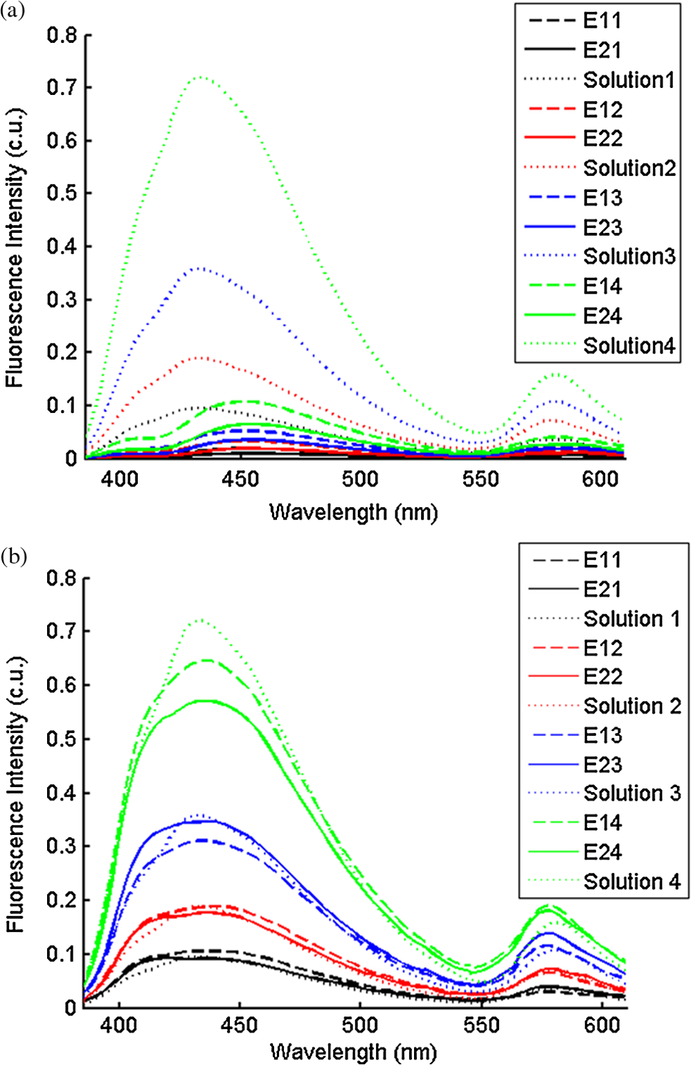 Figure 8(a) and 8(b) show the extraction of fluorophore concentrations of both fluorophores in phantom set E using the extracted fluorescence spectrum from phantom E21 as the known calibration standard (390- to 550-nm region for Stilbene and 550- to 610-nm region for Rhodamine). Figure 8(c) and 8(d) show the same data using phantom A21 as the calibration standard for Stilbene concentration extraction and phantom B21 for Rhodamine concentration extraction. Given that the excitation wavelength used in phantom set E was different from that in phantom set A (for Stilbene) and B (for Rhodamine), the extracted concentrations in Fig. 8(c) and 8(d) were calculated through the relationship to account for fluorophore absorbance as well as photon energy difference at different excitation wavelengths, where and are the fluorophore absorbance at the excitation wavelength of the target and calibration phantom, while and are the individual photon energy () at the excitation wavelength of the target and calibration phantom, respectively. The mean concentration extraction errors and standard deviations in Fig. 8(a) to 8(d) were , , , and , respectively, indicating the fluorophore concentration can be extracted with high accuracy when using an appropriate calibration standard regardless of whether the calibration phantom is excited at the same or different wavelength as the target phantom.Fig. 8(a) to (b) shows the extracted Stilbene and Rhodamine concentrations for each phantom subset (* and o) in set E using the 390- to 550-nm (for Stilbene) and 550- to 610-nm (for Rhodamine) regions of the extracted fluorescence spectrum of phantom E21 as the calibration standard. Also shown in these two figures are the extracted fluorophore concentrations of the corresponding non-turbid solutions () using the fluorescence of the solution with the lowest concentration as calibration standard. (c) and (d) show the extracted Stilbene and Rhodamine concentrations for each phantom subset in set E using the extracted intrinsic fluorescence spectrum of phantom A21 (for Stilbene) and B21 (for Rhodamine), respectively, as the calibration standards. The expected values are the true fluorophore concentration values. The dashed line in each figure indicates line of perfect agreement. 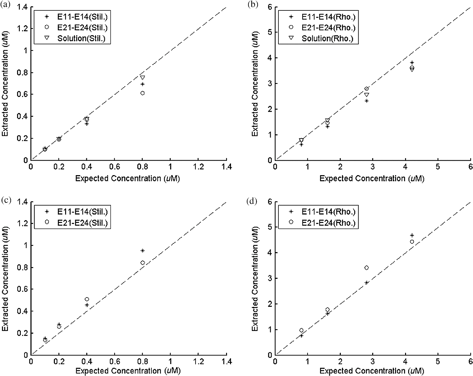 Figure 9 shows measured [Fig. 9(a) and 9(b)] and extracted [Fig. 9(c) and 9(d)] fluorescence from phantoms with odd [Fig. 9(a) and 9(c)] and even [Fig. 9(b) and 9(d)] number fluorophore concentrations (-- and -) in set F along with a linear combination of the measured fluorescence (implemented in post-processing) from two separate non-turbid fluorophore solutions containing each of the fluorophores (:). The same color indicates the same fluorophore concentration. As in Fig. 7, the intensity and shape differences between the two measured phantom spectra from each subset that have the same fluorophore concentration but different optical properties are corrected in the extracted fluorescence spectra. Compared with Fig. 7, it is not as straightforward to differentiate the two fluorophores here due to their overlapping emission regions (550 to 620 nm). In Fig. 9(c) and 9(d), as the fluorophore concentration increases, the measured fluorescence of the non-turbid fluorophore solution combination deviates more from the two phantom extracted spectra that have the same fluorophore concentration (: compared with -- and -). This is likely due to the fact that extracted intrinsic fluorescence is corrected for fluorophore reabsorption, whereas this is not the case in the non-turbid fluorophore solution, where as the concentration of fluorophore increases there is significant reabsorption, which is not corrected for. Fig. 9(a) and (b) Measured fluorescence from phantoms with odd (a) and even (b) number fluorophore concentrations (-- and -) in set F along with a linear combination of the measured fluorescence (implemented in post-processing) from two separate non-turbid fluorophore solutions containing each of the fluorophores (:); (c) and (d) Equivalent of (a) and (b), the only difference is the measured fluorescence from the phantoms is substituted by the corresponding extracted fluorescence. The same color indicates the same fluorophore concentration. (Color online only.)  Since 2-NBDG emits between 500 to 550 nm with no emission from Rhodamine in this wavelength range, the measured fluorescence between 500 to 550 nm was assigned to 2-NBDG fluorescence, which can then be used to extrapolate the intensity over 550 to 620 nm (the intensity at 540 nm was used for this purpose and the intensity between 550 to 620 nm was calculated based on their relative intensity ratios to that at 540 nm from the normalized 2-NBDG spectrum). Rhodamine fluorescence was then obtained by subtracting the 2-NBDG component from the two-component fluorescence spectrum. Once the two component spectra were separated, their concentrations were extracted using appropriate calibration phantoms. Figure 10(a) and 10(b) show the extraction of phantom fluorophore concentrations for both fluorophores from their separated extracted fluorescence spectrum using phantom F21 as the known calibration standard. Interestingly, the extracted intrinsic fluorescence has a much wider linear range than the measured non-turbid solution fluorescence. This is likely due to the fact that extracted intrinsic fluorescence is corrected for fluorophore reabsorption whereas that of the non-turbid fluorescence solution is not. Figure 10(c) and 10(d) show concentrations for both fluorophores using phantom C21 as the calibration standard for 2-NBDG and phantom B21 for Rhodamine. The fluorophore absorbance as well as photon energy differences were accounted for in the same way as mentioned previously when using B21 as calibration standard for Rhodamine concentration extraction since the excitation wavelengths are different between the two phantom sets. It is to be noted that the model in its current form does not account for fluorescence from one fluorophore as an excitation source for another; i.e., it does not separate Rhodamine fluorescence excited by NBDG fluorescence re-absorption from that excited by the instrument light source. The fluorescence of Rhodamine B in the target phantom is excited by both the instrument light source and NBDG fluorescence, while the reference phantom fluorescence is only excited by the light source of the instrument. Thus the extracted Rhodamine B concentration in Fig. 10(d) is higher than expected at higher concentrations partially because of reabsorption of NBDG fluorescence. Fig. 10(a) and (b) show the extracted 2-NBDG and Rhodamine concentrations for each phantom subset (* and o) in set F using separated 2-NBDG and Rhodamine fluorescence from the extracted fluorescence spectrum of phantom F21 as calibration standard. Also shown in these two figures are the extracted fluorophore concentrations of the corresponding non-turbid solutions () using the measured solution fluorescence of the lowest concentration as calibration standard. (c) and (d) show the extracted 2-NBDG and Rhodamine concentrations for each phantom subset in set F using the extracted fluorescence spectrum from phantom C21 (for 2-NBDG) and B21 (for Rhodamine), respectively, as the calibration standard. The expected values are the true fluorophore concentration values. The dashed line in each figure indicates line of perfect agreement. 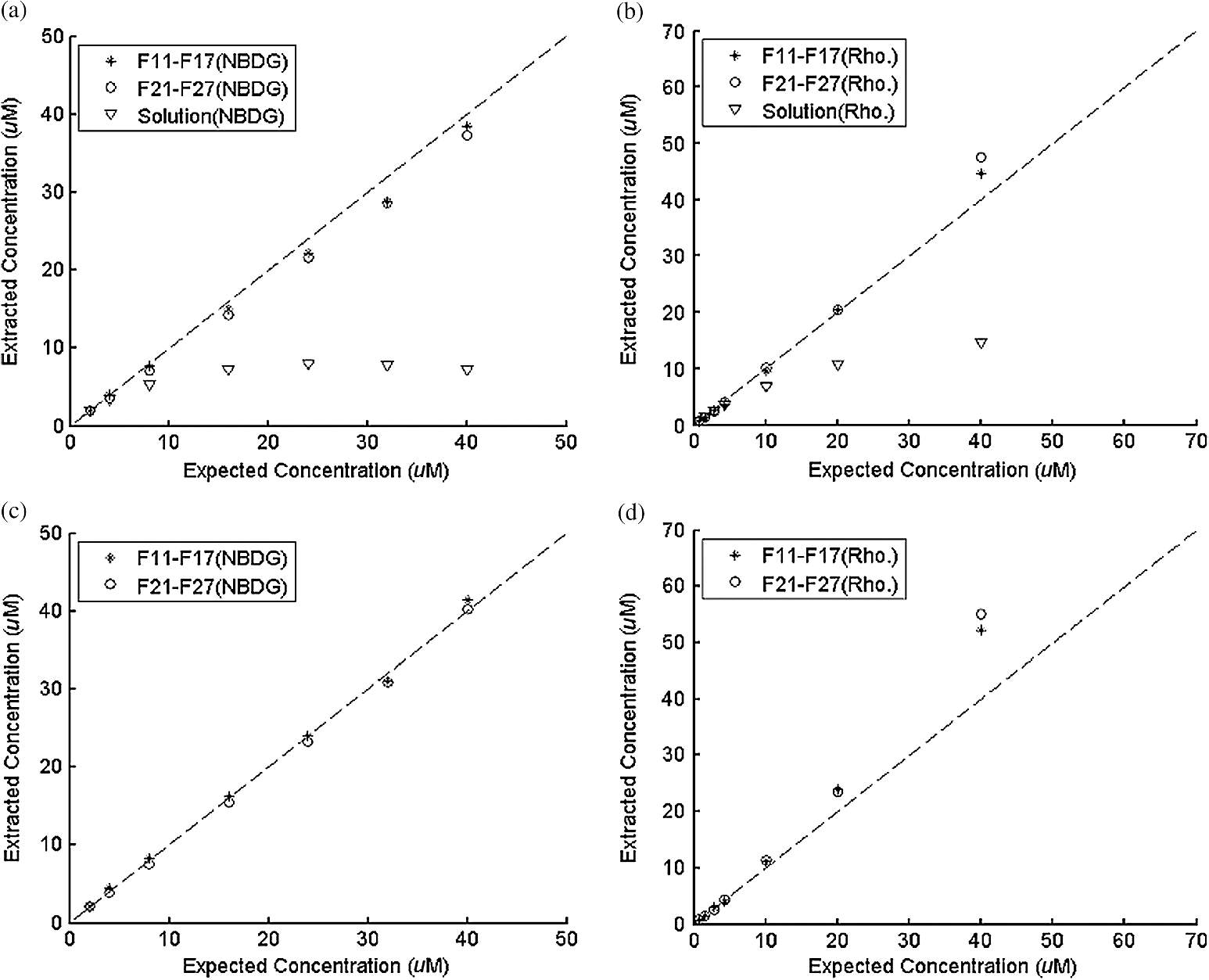 3.4.Pre-Clinical Pilot StudyFigure 11 shows measured and extracted fluorescence spectra at different time points for one mouse from the 6 mM 2-NBDG group. Figure 11(a) shows measured fluorescence spectra at four time points (baseline, t20, t40, and t60), and Fig. 11(b) shows the same data for the extracted fluorescence. The baseline fluorescence originates from RFP, while the fluorescence of the post-injection time points contains the contribution from both 2-NBDG and RFP. In both figures, fluorescence first increases after 2-NBDG injection and then decreases progressively as would be expected.43 The fluorophore emission features/peaks (545 nm for 2-NBDG and 575 nm for RFP) can easily be observed from distortion corrected (extracted) intrinsic fluorescence as compared with that in measured fluorescence, where the peaks are affected by the alpha and beta bands absorption of . Fig. 11Measured (a) and extracted (b) fluorescence spectra of four time points (baseline, t20, t40, and t60) for one animal from the 6 mM 2-NBDG group. Baseline corresponds to the time point before 2-NBDG injection, and t20, t40, and t60 mean 20, 40, and 60 min post 2-NBDG injection. (Color online only.)  Figure 12(a) shows the measured fluorescence intensity change over time, and Fig. 12(b) shows the same data for extracted intrinsic fluorescence for all mice. Figure 12(c) shows the mean and standard deviation of measured fluorescence spectra for each dose group, and Fig. 12(d) shows the same data for extracted fluorescence. The 2-NBDG peak fluorescence wavelength (545 nm) was used at each time point for all plots. For a given 2-NBDG dose, the measured and extracted fluorescence first increase to a maximum and then decreases due to 2-NBDG uptake by the cells.43 More importantly, there is a progressively increasing trend with increasing 2-NBDG dose in the extracted intrinsic fluorescence. However, this is much less significant in the raw fluorescence. The fluorescence measurements typically begin immediately after injection, which allows for the capture of both the rapid rise and fall off. There is one animal (dotted blue curve of 6 mM), however, that has different kinetics from the rest; i.e., the curve starts to decay almost immediately. This is due to the fact that there was a slight delay caused by probe movement, which prevented collected of data that shows the full extent of the rise. Fig. 12(a) shows the measured fluorescence intensity change over time for all mice, and (b) shows the same data for extracted fluorescence; (c) shows the mean and standard deviation of measured fluorescence spectra for each dose group, and (d) shows the same data for extracted fluorescence. Time point 0 is the time when 2-NBDG was injected. The legend indicates the injected 2-NBDG concentration. (Color online only.) 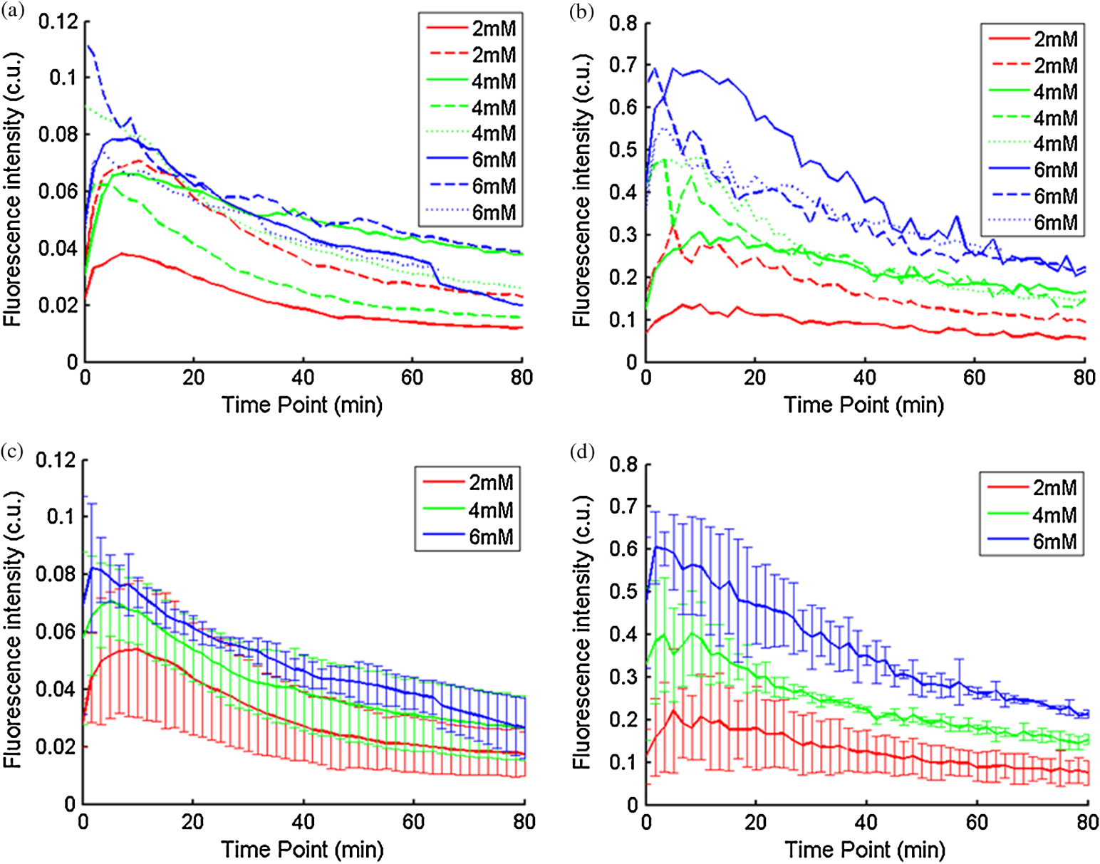 Figure 13 shows measured raw and extracted intrinsic fluorescence over injected 2-NBDG concentration for all mice. Figure 13(a) shows the scatter plot of measured fluorescence intensity as a function of injected 2-NBDG dose at three time points (t20, t40, and t60), and Fig. 13(b) shows the same data for extracted intrinsic fluorescence for all mice. The peak 2-NBDG fluorescence wavelength (545 nm) was used for each data point. The error bar indicates the standard deviation in each 2-NBDG concentration group. The value at the top of each figure is the Pearson’s linear correlation coefficient of the three doses at each time point and the coordinate origin (0,0). For a doubling or even tripling of the dose, the extracted fluorescence increases linearly while that of the measured fluorescence is non-linear with dose. Moreover, variations within the same dose group are smaller for intrinsic fluorescence than that for the measured fluorescence. Fig. 13(a) shows the scatter plot of measured fluorescence intensity over injected 2-NBDG concentration at three time points (t20, t40, and t60) for all the mice. (b) shows the same data for extracted fluorescence. The error bar shows the standard deviation among the mice in each 2-NBDG concentration group. The r value at the top of each figure indicates the linearity of the axis values over injected 2-NBDG concentrations (more linear when r approaches 1). t20, t40, and t60 mean 20, 40, and 60 min post-2-NBDG injection. (Color online only.) 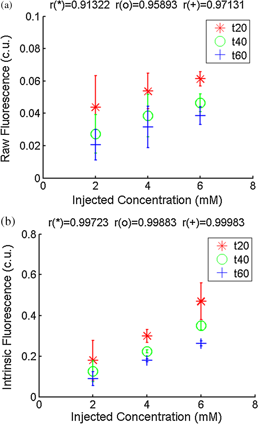 4.ConclusionsIn summary, the inverse Monte Carlo model developed previously by our group was validated experimentally to extract intrinsic fluorescence from biological meaningful single and multiple fluorophores in turbid media over a wide wavelength range that spans the UV and visible spectral range. It was shown that the model can restore intrinsic fluorescence shape with high accuracy and also has the capability to extract fluorophore concentration when calibrated to an appropriate reference phantom containing the same fluorophore and with known concentration. The significance of shape correction is that it can provide more reliable information of true media constituents, while fluorophore concentration extraction will provide quantitative tissue concentrations of biochemical constituents, therefore aiding in the proper interpretation of the tissue spectra. The value/merit of the model has been demonstrated in a pilot animal study. It was shown that after model correction, the fluorophore emission features/peaks of 2-NBDG, an optical analog to FDG can easily be observed from distortion corrected intrinsic fluorescence. A strong linear correlation exists between intrinsic fluorescence and injected 2-NBDG dose, and different groups of dose injection can be separated from each other based on the corrected fluorescence. Quantitative diffuse reflectance spectroscopy of tissues using an inverse Monte Carlo model of reflectance has also been developed by our group40 and shown to accurately extract total hemoglobin concentration (marker of tissue vascularity), and oxygen saturation (marker of tissue vascular oxygenation).11,51,52,54 The overall strategy of diffuse reflectance and fluorescence spectroscopy using our scalable inverse Monte Carlo models is to ultimately provide a powerful tool to quantitatively, rapidly and non-destructively examine bioenergetics of living tissues and in particular, cancers by simultaneously being able to report on the three axes of energy production: vascular oxygenation, mitochondrial activity (TMR), and glycolysis (2-NBDG, NADH). AcknowledgmentsThis work was funded by DOD grant W81XWH-09-1-0410. Chengbo Liu also wants to thank China Scholarship Council for supporting his two years research at Duke University as well as the support from NSFC grant 61120106013. Karthik Vishwanath is grateful for receiving financial support from the NIH (Grant: 5K99CA140783-02). ReferencesN. Ramanujam,
“Fluorescence spectroscopy in vivo,”
Encyclopedia of Analytical Chemistry, 20
–56 John Wiley and Sons, Ltd., Chichester
(2000). Google Scholar
Q. Fanget al.,
“Time-domain laser-induced fluorescence spectroscopy apparatus for clinical diagnostics,”
Rev. Sci. Instrum., 75
(1), 151
–162
(2004). http://dx.doi.org/10.1063/1.1634354 RSINAK 0034-6748 Google Scholar
K. Sokolovet al.,
“Opitcal spectroscopy for detection of neoplasia,”
Curr. Opin. Chem. Biol., 6
(5), 651
–658
(2002). http://dx.doi.org/10.1016/S1367-5931(02)00381-2 COCBF4 1367-5931 Google Scholar
A. Shahzadet al.,
“Diagnostic application of fluorescence spectroscopy in oncology field: hopes and challenges,”
Appl. Spectros. Rev., 45
(1), 92
–99
(2010). http://dx.doi.org/10.1080/05704920903435599 APSRBB 0570-4928 Google Scholar
W. J. CottrellA. R. OseroffT. H. Foster,
“Portable instrument that integrates irradiation with fluorescence and reflectance spectroscopies during clinical photodynamic therapy of cutaneous disease,”
Rev. Sci. Instrum., 77
(6), 064302
(2006). http://dx.doi.org/10.1063/1.2204617 RSINAK 0034-6748 Google Scholar
P. Hillemannset al.,
“Photodetection of cervical intraepithelial neoplasia using 5-aminolevulinic acid-induced porphyrin fluroescence,”
Cancer, 88
(10), 2275
–2282
(2000). http://dx.doi.org/10.1002/(ISSN)1097-0142 CANCAR 1097-0142 Google Scholar
C. Kurachiet al.,
“Fluorescence spectroscopy for the detection of tongue carcinoma-validation in an animal model,”
Biomed. Opt., 13
(3), 034018
(2008). http://dx.doi.org/10.1117/1.2937214 BOEICL 2156-7085 Google Scholar
L. Coghlanet al.,
“Fluorescence spectroscopy of epithelial tissue throughout the dysplasia-carcinoma sequence in an animal model: spectroscopic changes precede morphologic changes,”
Laser. Surg. Med., 29
(1), 1
–10
(2001). http://dx.doi.org/10.1002/(ISSN)1096-9101 LSMEDI 0196-8092 Google Scholar
Z. Volynskayaet al.,
“Diagnosing breast cancer using diffuse reflectance spectroscopy and intrinsic fluorescence spectroscopy,”
Biomed. Opt., 13
(2), 024012
(2008). http://dx.doi.org/10.1117/1.2909672 BOEICL 2156-7085 Google Scholar
H. J. C. M. Sterenborget al.,
“In vivo fluorescence spectroscopy and imaging of human skin tumours,”
Laser. Med. Sci., 9
(3), 191
–201
(1994). Google Scholar
C. Zhuet al.,
“Diagnosis of breast cancer using fluorescence and diffuse reflectance spectroscopy: a Monte-Carlo-model-based approach,”
Biomed. Opt., 13
(3), 034015
(2008). http://dx.doi.org/10.1117/1.2931078 BOEICL 2156-7085 Google Scholar
B. Chanceet al.,
“Oxidation-reduction ratio studies of mitochondria in freeze-trapped samples,”
J. Biol. Chem., 254
(11), 4764
–4771
(1979). BCHSEI 0177-3593 Google Scholar
B. Chanceet al.,
“Mitochondrial NADH as the bellwether of tissue O2 delivery,”
Adv. Exp. Med. Biol., 566 231
–242
(2005). http://dx.doi.org/10.1007/b137055 AEMBAP 0065-2598 Google Scholar
G. A. Wagniereset al.,
“In vivo fluorescence spectroscopy and imaging for oncological applications,”
Photochem. Photobiol., 68
(5), 603
–632
(1998). PHCBAP 0031-8655 Google Scholar
T. CornbleetH. Popper,
“Properties of human skin revealed by fluorescence microscopy: the normal skin; the vitamin A content of the skin,”
Arch. Dermatol., 46
(1), 59
–65
(1942). http://dx.doi.org/10.1001/archderm.1942.01500130062005 ARDEAC 0003-987X Google Scholar
R. GreenbergH. Popper,
“Demonstration of Vitamin A in the retina by fluorescence microscopy,”
Am. J. Physiol., 134
(1), 0114
–0118
(1941). Google Scholar
R. A. Schwarz, Department of Bioengineering, Rice University, Houston
(2010). Google Scholar
G. Palmeret al.,
“Non-invasive monitoring of intra-tumor drug concentration and therapeutic response using optical sepctroscopy,”
J. Contr. Release, 142
(3), 457
–464
(2010). http://dx.doi.org/10.1016/j.jconrel.2009.10.034 JCREEC 0168-3659 Google Scholar
R. Richards-Kortumet al.,
“Acetic acid as a signal enhancing contrast agent in fluorescence spectroscopy,”
Lifespex, Inc., USA
(2001). Google Scholar
A. Pelegrinet al.,
“Antibody-fluorescein conjugates for photoimmunodiagnosis of human colon carcinoma in nude mice,”
Cancer, 67
(10), 2529
–2537
(1991). http://dx.doi.org/10.1002/(ISSN)1097-0142 CANCAR 1097-0142 Google Scholar
K. Sakataniet al.,
“Noninvasive optical imaging of the subarachnoid space and cerebrospinal fluid pathways based on near-infrared fluorescence,”
J. Neurosurg., 87
(5), 738
–745
(1997). http://dx.doi.org/10.3171/jns.1997.87.5.0738 JONSAC 0022-3085 Google Scholar
N. Rajaramet al.,
“Design and validation of a clinical instrument for spectral diagnosis of cutaneous malignancy,”
Appl. Opt., 49
(2), 142
–152
(2010). http://dx.doi.org/10.1364/AO.49.000142 APOPAI 0003-6935 Google Scholar
Y. FawzyH. J. Zeng,
“Intrinsic fluorescence spectroscopy for endoscopic detection and localization of the endobronchial cancerous lesions,”
Biomed. Opt., 13
(6), 064022
(2008). http://dx.doi.org/10.1117/1.3041704 BOEICL 2156-7085 Google Scholar
I. GeorgakoudiB. C. JacobsonM. G. Muller,
“NAD(P)H and collagen as in vivo quantitative fluorescent biomarkers of epithelial precancerous changes,”
Cancer Res., 62
(3), 682
–687
(2002). CNREA8 0008-5472 Google Scholar
G. M. Palmeret al.,
“Quantitative diffuse reflectance and fluorescence spectroscopy: a tool to monitor tumor physiology in vivo,”
Biomed. Opt., 14
(2), 024010
(2009). http://dx.doi.org/10.1117/1.3103586 BOEICL 2156-7085 Google Scholar
J. C. FinlayT. H. Foster,
“Recovery of hemoglobin oxygen saturation and intrinsic fluorescence with a forward-adjoint model,”
Appl. Opt., 44
(10), 1917
–1933
(2005). http://dx.doi.org/10.1364/AO.44.001917 APOPAI 0003-6935 Google Scholar
N. C. Biswal,
“Recovery of turbidity free fluroescence from measured fluorescence: an experimental approach,”
Opt. Express, 11
(24), 3320
–3331
(2003). http://dx.doi.org/10.1364/OE.11.003320 OPEXFF 1094-4087 Google Scholar
R. Weersinket al.,
“Noninvasive measurement of fluorophore concentration in turbid media with a simple fluorescence/reflectance ratio technique,”
Appl. Opt., 40
(34), 6389
–6395
(2001). http://dx.doi.org/10.1364/AO.40.006389 APOPAI 0003-6935 Google Scholar
V. S. RajaS. GuptaA. Pradhan,
“Recovery of intrinsic fluorescence of tissue mimicking model media and human breast tissues from spatially resolved fluorescence and simultaneous evaluation of optical transport parameters,”
Proc. SPIE, 6091 609104
(2006). http://dx.doi.org/10.1117/12.645918 PSISDG 0277-786X Google Scholar
K. R. DiamondT. J. FarrellM. S. Patterson,
“Measurement of fluorophore concentrations and fluorescence quantum yield in tissue-simulating phantoms using three diffusion models of steady-state spatially resolved fluorescence,”
Phys. Med. Biol., 48
(24), 4135
–4149
(2003). http://dx.doi.org/10.1088/0031-9155/48/24/011 PHMBA7 0031-9155 Google Scholar
R. Drezek,
“Understanding the contributions of NADH and collagen to cervical tissue fluorescence spectra: modeling, measurements, and implications,”
Biomed. Opt., 6
(4), 385
–396
(2001). http://dx.doi.org/10.1117/1.1413209 BOEICL 2156-7085 Google Scholar
M. G. Mulleret al.,
“Intrinsic fluorescence spectroscopy in turbid media: disentangling effects of scattering and absorption,”
Appl. Opt., 40
(25), 4633
–4646
(2001). http://dx.doi.org/10.1364/AO.40.004633 APOPAI 0003-6935 Google Scholar
Q. Zhanget al.,
“Turbidity-free fluorescence spectroscopy of biological tissue,”
Opt. Lett., 25
(19), 1451
–1453
(2000). http://dx.doi.org/10.1364/OL.25.001451 OPLEDP 0146-9592 Google Scholar
J. WuM. S. FeldR. P. Rava,
“Analytical model for extracting intrinsic fluorescence in turbid media,”
Appl. Opt., 32
(19), 3585
–3595
(1993). http://dx.doi.org/10.1364/AO.32.003585 APOPAI 0003-6935 Google Scholar
S. K. Changet al.,
“Model-based analysis of clinical fluorescence spectroscopy for in vivo detection of cervical intraepithelial dysplasia,”
Biomed. Opt., 11
(2), 024008
(2006). http://dx.doi.org/10.1117/1.2187979 BOEICL 2156-7085 Google Scholar
W. M. Star,
“Diffusion theory of light transport,”
Optical-Thermal Response of Laser-Irradiated Tissue, 145
–202 Springer, New York
(1995). Google Scholar
L. WangS. L. JacquesL. Zheng,
“MCML-Monte Carlo modeling of light transport in multi-layered tissues,”
Comput. Meth. Prog. Bio., 47
(2), 131
–146
(1995). http://dx.doi.org/10.1016/0169-2607(95)01640-F CMPBEK 0169-2607 Google Scholar
I. J. Georgakoudi,
“The color of cancer,”
J. Lumin., 119–120 75
–83
(2006). Google Scholar
D. YudovskyL. Pilon,
“Modeling the local excitation fluence rate and fluorescence emission in absorbing and strongly scattering multilayered media,”
Appl. Opt., 49
(31), 6072
–6084
(2010). http://dx.doi.org/10.1364/AO.49.006072 APOPAI 0003-6935 Google Scholar
G. M. PalmerN. Ramanujam,
“Monte Carlo-based inverse model for calculating tissue optical properties. Part I: Theory and validation on synthetic phantoms,”
Appl. Opt., 45
(5), 1062
–1071
(2006). http://dx.doi.org/10.1364/AO.45.001062 APOPAI 0003-6935 Google Scholar
G. M. PalmerN. Ramanujam,
“Monte-Carlo-based model for the extraction of intrinsic fluorescence from turbid media,”
Biomed. Opt., 13
(2), 024017
(2008). http://dx.doi.org/10.1117/1.2907161 BOEICL 2156-7085 Google Scholar
A. G. Dawson,
“Oxidation of cytosolic NADH formed during aerobic metabolism in mammalian cells,”
Trends Biochem. Sci., 4
(8), 171
–176
(1979). http://dx.doi.org/10.1016/0968-0004(79)90417-1 TBSCDB 0167-7640 Google Scholar
S. R. Millonet al.,
“Uptake of 2-NBDG as a method to monitor therapy response in breast cancer cell lines,”
Breast Cancer Res. Treat., 126
(1), 55
–62
(2011). BCTRD6 Google Scholar
R. C. ScadutoL. W. Grotyohann,
“Measurement of mitochondrial membrane potential using fluorescent rhodamine derivatives,”
Biophys. J., 76
(1), 469
–477
(1999). http://dx.doi.org/10.1016/S0006-3495(99)77214-0 BIOJAU 0006-3495 Google Scholar
J. E. Benderet al.,
“A robust Monte Carlo model for the extraction of biological absorption and scattering in vivo,”
IEEE Trans. Biomed. Eng., 56
(4), 960
–968
(2009). http://dx.doi.org/10.1109/TBME.2008.2005994 IEBEAX 0018-9294 Google Scholar
K. Vishwanathet al.,
“Portable, fiber-based, diffuse reflectance spectroscopy (DRS) systems for estimating tissue optical properties,”
Appl. Spectros., 62
(2), 206
–215
(2011). http://dx.doi.org/10.1366/10-06052 APSPA4 0003-7028 Google Scholar
S. Prahl, Mie Scattering Program, Oregon Med. Laser Center, Oregon,
(2005). Google Scholar
M. R. Duchen,
“Mitochondrial function in Type I cells isolated from rabbit arterial chemoreceptors,”
J. Physiol., 450 13
–31
(1992). JJPHAM 0021-521X Google Scholar
K. Vishwanathet al.,
“Using optical spectroscopy to longitudinally monitor physiological changes within solid tumors,”
Neoplasia, 11
(9), 889
–900
(2009). 1522-8002 Google Scholar
C. Zhu,
“Diagnosis of breast cancer using diffuse reflectance spectroscopy: comparison of a Monte Carlo versus partial least squares analysis based feature extraction technique,”
Laser. Surg. Med., 38
(3), 714
–724
(2006). Google Scholar
V. T. Changet al.,
“Quantitative physiology of the precancerous cervix in vivo through optical spectroscopy,”
Neoplasia, 11
(4), 325
–332
(2009). 1522-8002 Google Scholar
B. YuH. FuN. J. Ramanujam,
“Instrument independent diffuse reflectance spectroscopy,”
Biomed. Opt., 16
(1), 011010
(2011). http://dx.doi.org/10.1117/1.3524303 BOEICL 2156-7085 Google Scholar
K. Vishwanathet al.,
“Quantitative optical spectroscopy can identify long-term local tumor control in irradiated murine head and neck xenografts,”
Biomed. Opt., 14
(5), 054051
(2009). http://dx.doi.org/10.1117/1.3251013 BOEICL 2156-7085 Google Scholar
|
|||||||||||||||||||||||||||||||||||||||||||||||||||||||||||||||||||||||||||||||||||||||||||||||||||||||||||||||||||||||||||||||||||||||||||||||||||||||||||||||||||