Nonlinear motion compensation using cubature Kalman filter for in vivo fluorescence microendoscopy in peripheral lung cancer intervention

Tiancheng He; Zhong Xue; Miguel Valdivia y Alvarado; Kelvin K. Wong; Weixin Xie; Stephen T. C. Wong

doi:10.1117/1.JBO.18.1.016008

7 January 2013 Nonlinear motion compensation using cubature Kalman filter for in vivo fluorescence microendoscopy in peripheral lung cancer intervention

Tiancheng He, Zhong Xue, Miguel Valdivia y Alvarado, Kelvin K. Wong, Weixin Xie, Stephen T. C. Wong

Author Affiliations +

Journal of Biomedical Optics, Vol. 18, Issue 1, 016008 (January 2013). https://doi.org/10.1117/1.JBO.18.1.016008

Abstract

Fluorescence microendoscopy can potentially be a powerful modality in minimally invasive percutaneous intervention for cancer diagnosis because it has an exceptional ability to provide micron-scale resolution images in tissues inaccessible to traditional microscopy. After targeting the tumor with guidance by macroscopic images such as computed tomorgraphy or magnetic resonance imaging, fluorescence microendoscopy can help select the biopsy spots or perform an on-site molecular imaging diagnosis. However, one challenge of this technique for percutaneous lung intervention is that the respiratory and hemokinesis motion often renders instability of the sequential image visualization and results in inaccurate quantitative measurement. Motion correction on such serial microscopy image sequences is, therefore, an important post-processing step. We propose a nonlinear motion compensation algorithm using a cubature Kalman filter (NMC-CKF) to correct these periodic spatial and intensity changes, and validate the algorithm using preclinical imaging experiments. The algorithm integrates a longitudinal nonlinear system model using the CKF in the serial image registration algorithm for robust estimation of the longitudinal movements. Experiments were carried out using simulated and real microendoscopy videos captured from the CellVizio 660 system in rabbit VX2 cancer intervention. The results show that the NMC-CKF algorithm yields more robust and accurate alignment results.

1. Introduction

Confocal fluorescence microendoscopy with molecular labeling plays an important role in analyzing cellular morphometry and activity at the molecular level for specimen investigation. Compared to traditional and intravital microscopy, confocal fluorescence microendoscopy can assess deep tissues in vivo by using a fiber-optic probe while providing microscopic-level resolution. In this way, it is possible to access internal organs with minimally invasive intervention techniques. In animal-based cancer research, this technology enables researchers to detect cancerous tissues, to discern the expression of specific genes using different auxiliary dyes, and to observe tumor growth and treatment responses. It can also be applied to studying sarcomeres, synapses, and glial cell activities in vivo.¹^–³

In lung cancer applications, in vivo detection of fluorescence-labeled tumor cells coupled with image-guided intervention have added new dimensions for on-site peripheral lung cancer diagnosis⁴^–⁷ due to its extraordinary ability of providing micron-scale resolution images in tissues inaccessible to light microscopy.⁸^,⁹ In clinical applications, traditional computed tomography (CT) appears to result in high false positive rates, and further biopsy is often necessary to confirm suspected cancer, particularly for small tumors. Image-guided microendoscopy, therefore, can accurately target small early stage tumors, detect the existence of cancerous tissues at microscopic resolution, and help select biopsy spots to perform on-site diagnosis. To detect cancerous tissues with fluorescence microendoscopy, various contrast agents can be used. One example is that, by injecting the fluorescent dye IntegriSense 680 (PerkinElmer, Inc., Waltham, Massachusetts) to label $α_{v} β_{3}$ integrin, cancerous tissues can be highlighted and detected by the microendoscopy system.¹⁰

In vivo fluorescent microendoscopy images are often affected by respiratory and hemokinesis motion, resulting in unstable visualization and quantitative measurement of the contrast agent expression, even when the interventional probe is immobilized.¹¹ For example, in lung cancer intervention, after the fiber-optic needle tip is successfully guided into the tumor, the microendoscopy image sequences will demonstrate periodic fluctuation induced by respiratory and heart systole.¹² Therefore, motion correction on the microendoscopy image sequence clips helps improve the visualization and quantification of tissue characteristics. Such motion correction or image registration among sequential images or a stack of images is a common post-processing task in other in vivo microscopic image acquisitions. Thus, in this paper, we focus on developing a motion correction algorithm for serial microscopic image sequences to compensate for periodic spatial deformation and intensity changes.

In the literature, many image computing methods¹³^–¹⁷ are proposed to alleviate the effect of periodical respiratory motion disturbance presented in microendoscopy videos. Global or local serial image alignment, also known as image registration, aims to determine the transformation with proper constraints by optimizing image similarity measures such as cross-correlation, mutual information, or squared intensity differences. In the meantime, geometric transformations such as scaling, affine, and elastic deformations are adopted to model the longitudinal movement across the microendoscopy video. In 2009, for example, Greenberg and Kerr¹⁵ proposed an algorithm based on the Lucas-Kanade algorithm. The approach estimates the line-by-line offsets by minimizing the squared intensity difference between each line in the reference frame and the corresponding line in its subsequent frames using the gradient descent method. A hidden Markov model (HMM)–based algorithm was also proposed to employ a smoothness constraint on the offsets of temporally corresponding lines for motion tracking.¹⁴^,¹⁸ However, these methods correct the motion disturbance line by line, an approach suitable only for line-based, laser scanning, intra-vital microscopy. An alternative method is to eliminate the undesired movement of the microendoscopy probe during imaging. Huang et al.¹⁹ investigated a motion-compensated, fiber-optic confocal microscope system for Fourier domain common-path optical coherence tomography (CP-OCT). They employed peak detection of a 1-D A-scan data of CP-OCT to monitor the distance deviation from the focal plane and then used a linear motor to drive the confocal microscope probe into a predetermined limit. Unfortunately, even though this method focuses on eliminating the unwanted probe movement, it cannot annotate the complexity of the nonlinear motion within microendoscopy videos.

In order to quantitatively analyze and precisely measure the fluorescence signals in microendoscopy videos for peripheral lung tumor diagnosis at the molecular level,²⁰^,²¹ we propose a nonlinear motion compensation algorithm using a cubature Kalman filter (NMC-CKF) which aims to correct the periodic respiratory motion. A longitudinal nonlinear system model using CKF is adopted to improve the temporal stability of the motion signals. The temporal motion can be restored by iteratively estimating the temporal transformations and applying CKF filtering to these transformations. Compared to the methods that only register the subsequent frames with the reference image, the NMC-CKF algorithm can generate more accurate registration results because it simulates the innate nonlinear property of the microendoscopy videos.

Using animal imaging data, two sets of experiments were carried out to evaluate the performance of the proposed NMC-CKF algorithm. The first experiment validated the algorithm with simulated microscopy image sequences by recovering the longitudinal transformations and comparing them with the ground truth. We compared the performance of the algorithm using three different image similarity measures with and without the CKF filtering. The results showed that the NMC-CKF using normalized mutual information (NMI) yielded more accurate estimation of the simulated transformations. The second set of the experiments applied the proposed algorithm to real microendoscopy image sequences collected by the CellVizio 660 system during our rabbit lung intervention experiments. The NMC-CKF algorithm with NMI image similarity measure and the NMI-based motion correction without CKF were compared. The results demonstrated that our algorithm yielded smaller image intensity differences after motion correction.

The remainder of this paper is organized as follows: Sec. 2 introduces the proposed NMC-CKF algorithm. Section 3 presents the experimental results. Finally, Sec. 4 summarizes and concludes our study.

2. Methods

2.1.

Need for Microendoscopy Motion Compensation in Intervention

Serial microscopic images captured during confocal fluorescence microendoscopy for in vivo applications are subject to spatial shifts, nonlinear deformations, and intensity changes due to respiratory and hemokinesis motions. Therefore, as a post-processing step, it is necessary to perform sequential image alignments for improved visualization and quantitative analysis. In our recently developed, minimally invasive, image-guided system⁹ for guiding percutaneous lung intervention, we observed such motion from the microendoscopy image sequences. Figure 1(a) shows the system, while Fig. 1(b) demonstrates that after successfully targeting the lesion, the needle inside the cannula can be replaced with the CellVizio 660 fiber-optic microendoscopy probe, and the fluorescence images are captured for cancerous assessment. The workflow of the system has previously been described.⁹ In order to perform on-site diagnosis of lung cancer, the IntegriSense 680 fluorescent contrast agent is used to label $α_{v} β_{3}$ integrin expressed in malignant cancer cells, and fiber-optic microendoscopy is performed to capture the IntegriSense expression with real-time video. In this way, the tumor and normal tissue information on the tip of the fiber-optic probe can be captured. Figure 1(b) illustrates fiber-optic microendoscopy during intervention. The diameter of the fiber-optic probe is 1 mm and can be easily used to visualize the tissue through the cannula. Unfortunately, because of respiratory and hemokinesis motion, the morphology and intensities of the image sequences are subject to change, which in turn affects quantitative analysis of the microendoscopy video for automatic tumor detection. Therefore, the goal of this study is to develop an effective motion compensation for microendoscopy image sequences.

Fig. 1

The intervention system and on-the-spot optical microendoscopy. (a) (1) the intervention system; (2) needle puncturing the rabbit lung; (3) CellVizio 660 fiber-optic microendoscopy probe. (b) A cannula with needle is first placed to target the tumor using image guidance and then replaced by a fiber-optic probe for in vivo microendoscopy to obtain high-resolution optical imaging data.

2.2.

Traditional Image Similarity-Based Registration

Denoting the microendoscopy image sequence as $I = {I_{1}, I_{2}, \dots, I_{N}}$ , where $N$ is the number of frames, image similarity-based motion compensation recovers the longitudinal transformations by minimizing the frame-to-frame differences. The image similarity measure is denoted as $SIM (H_{t} \circ I_{t}, I_{t + 1})$ , where $H_{t} \circ I_{t}$ is the transformed frame $t$ to $t + 1$ using transformation $H_{t}$ . So, $H = {H_{1}, H_{2}, \dots, H_{N - 1}}$ stands for serial transformations. Based on applications, the similarity measure can be least squares (LS), cross-correlation (CroC), NMI, or others. The goal of the registration is to find the optimal longitudinal transformations $H$ by maximizing image similarity across the image sequence:

Eq. (1)

E_{1} (H) = \frac{1}{N - 1} \sum_{t = 1}^{N - 1} [SIM (H_{t} \circ I_{t}, I_{t + 1})] .

For our purpose, the transformation $H_{t}$ can be represented by a 5-D vector $h_{t} = {[h_{1}, \dots, h_{5}]}^{T}$ , consisting of translations in the $x$ - and $y$ -directions, rotation, and scaling, as well as the image intensity scaling between two image frames. The problem with using this traditional method is that the serial alignment parameters obtained from the image sequence are independent at different points in time and might be temporally unstable because there is no longitudinal information applied in the motion correction method. In this work, we proposed to incorporate the CKF model for more robust estimation of the longitudinal transformations.

2.3.

NMC-CKF Algorithm

In order to improve the temporal stability and accuracy of motion compensation, we propose the NMC-CKF algorithm. In this algorithm, the longitudinal transformation is regularized by both image similarity measures and a nonlinear system. Because the longitudinal transformations are subject to the constraints of the nonlinear system, the resultant longitudinal transformations are more robust and accurate compared to the frame-to-frame image registration. Figure 2 shows the flowchart of the proposed algorithm, and each step will be detailed next.

Fig. 2

The NMC-CKF flowchart. Given the input microendoscopy video, the NMC-CKF algorithm aligns the video by estimating the longitudinal transformations ( $H$ ) and the actual motion vectors ( $M$ ) iteratively. Finally, a deformable motion correction method is applied to fine-tune the nonlinear deformation across the video sequences.

2.3.1.

Incorporating the nonlinear system model in longitudinal transformations

In order to model $H$ , the longitudinal transformations obtained from image registration, we adopted a nonlinear system model. From the systems point of view, $H$ can be regarded as the output of a nonlinear system, whose states are the actual temporal transformations to be estimated. The system can be described as follows:

Eq. (2)

{\begin{cases} M_{t + 1} = f (M_{t}, u_{t + 1}) + n_{t + 1} \\ H_{t + 1} = g (M_{t + 1}) + w_{t + 1} \end{cases},

where

M

represents the system’s state,

u

is the system’s input,

n \in N (0, Q)

denotes the input noise,

w \in N (0, R)

stands for the measurement noise, and

f (\cdot)

is the nonlinear system function.²² The system output function

g (\cdot)

is assumed to be identity transformation, and the input signal

u

is assumed to be zero. Therefore,

H

can be considered to be an observation or the nonlinear system’s output, and

M

represents the actual motion vectors to be estimated. By combining such a nonlinear system with the similarity measurement-based image registration [in Eq. (1)], the motion compensation problem can be formulated by minimizing the following energy function:

Eq. (3)

E_{2} = \frac{1}{N - 1} \sum_{t = 1}^{N - 1} [SIM (H_{t} \circ I_{t}, I_{t + 1}) + α {‖ H_{t} - g (M_{t}) ‖}^{2}] .

We hypothesize that $M$ is the underlying longitudinal transformations that are more robust and accurate than $H$ because $H$ may fluctuate if they are solved directly by using image registration. In the first term of Eq. (3), the image similarity is evaluated using a similarity measure. According to the second term, the longitudinal transformation $H_{t}$ is subject to a regularization of the nonlinear system. This energy function can be iteratively minimized: first, assuming that $M$ is known, minimizing the similarity value leads to the transformation matrix $H$ , while making sure that $H$ is similar to $g (M)$ . Then, assuming that $H$ is known, the nonlinear system’s state $M$ can be calculated by applying the CKF algorithm to the nonlinear system described in Eq. (2).

Like the extended Kalman filter (EKF), CKF is a minimum mean-square error (MMSE) estimator specially designed for nonlinear systems. The difference between them is that CKF uses the spherical-radial rule²³ and makes it possible to numerically calculate the variability of system’s states, thereby simplifying the calculation of their covariance matrices. Hence, the advantage of CKF over EKF is that there is no calculation of the Jacobian and Hessian matrices of the system’s states.

According to CKF, the filtering procedure contains two iterative steps: the predicting and updating steps.²³ For initialization, $H$ obtained by minimizing Eq. (1) are regarded as the initial values of $M$ , and ${\hat{M}}_{t | t} (t = 1)$ can be initialized as the mean of $M$ across the time sequence. Then, the QR decomposition is used to factorize the covariance matrix $P_{t | t}$ of $M$ ; i.e., $P_{t | t} = R_{t | t} R_{t | t}^{T}$ , for $t = 1$ . The major steps for the NMC-CKF algorithm are summarized as follows.

a. Predicting the covariance matrix of the system states from $t$ to $t + 1$
- 1. Calculate the cubature points $ζ_{i, t | t} (i = 1, 2, \dots, m)$ at time $t$ by using
  Eq. (4)
  $ζ_{i, t | t} = R_{t | t} ξ_{i} + {\hat{M}}_{t | t},$
  where $m$ is the number of cubature points and is determined by the number of images $N$ [i.e., $m = 2 (N - 1)$ ], $ξ_{i} = - \sqrt{\frac{m}{2}}$ , for $i = 1, 3, 5, \dots, m - 1$ ; $\sqrt{\frac{m}{2}}$ , for $i = 2, 4, 6, \dots, m$ . It can be seen that the cubature points $ζ_{i, t | t}$ reflect the variability of $M$ .
- 2. Propagating the cubature points from time $t$ to $t + 1$ [i.e., $ζ_{i, t | t}^{*} = f (ζ_{i, t | t})$ ], $(i = 1, 2, \dots, m)$ can be estimated by using a linear prediction, and the predicted state ${\hat{M}}_{t + 1 | t}$ can be calculated as the mean of the propagated cubature points:
  Eq. (5)
  ${\hat{M}}_{t + 1 | t} = \frac{1}{m} \sum_{i = 1}^{m} ζ_{i, t + 1 | t}^{*} .$
- 3. The covariance matrix of the system’s states at time $t + 1$ , $P_{t + 1 | t}$ , can be predicted as
  Eq. (6)
  $P_{t + 1 | t} = \frac{1}{m} \sum_{i = 1}^{m} ζ_{i, t + 1 | t}^{*} ζ_{i, t + 1 | t}^{* T} - {\hat{M}}_{t + 1 | t} {\hat{M}}_{t + 1 | t}^{T} .$
b. Updating the covariance matrix of the system states for time $t + 1$
- 1. The covariance matrix $P_{t + 1 | t}$ can be factorized using the QR decomposition [i.e., $P_{t + 1 | t} = R_{t + 1 | t} R_{t + 1 | t}^{T}$ ], and the cubature points at time $t + 1$ can be calculated as $ζ_{i, t + 1 | t} = R_{t + 1 | t} ξ_{i} + {\hat{M}}_{t + 1 | t}$ , similar to Eq. (4). Then, the system output of the propagated cubature points can be written as $ψ_{i, t + 1 | t} = ζ_{i, t + 1 | t}$ .
- 2. Estimate the system output by using
  Eq. (7)
  ${\hat{H}}_{t + 1 | t} = \frac{1}{m} \sum_{i = 1}^{m} ψ_{i, t + 1 | t} .$
- 3. Calculating the covariance matrix of the system output, $P_{H H, t + 1 | t}$ , and the cross-covariance matrix of the system states and outputs, $P_{M H, t + 1 | t}$ :
  Eq. (8)
  $P_{H H, t + 1 | t} = \frac{1}{m} \sum_{i = 1}^{m} ψ_{i, t + 1 | t} ψ_{i, t + 1 | t}^{T} - {\hat{H}}_{t + 1 | t} {\hat{H}}_{t + 1 | t}^{T} and P_{M H, t + 1 | t} = \frac{1}{m} \sum_{i = 1}^{m} ζ_{i, t + 1 | t} ψ_{i, t + 1 | t}^{T} - {\hat{M}}_{t + 1 | t} {\hat{H}}_{t + 1 | t}^{T} .$
- 4. Calculate the Kalman gain at time $t + 1$ using $W_{t + 1} = P_{M H, t + 1 | t} P_{H H, t + 1 | t}^{- 1}$ , and update the system state using ${\hat{M}}_{t + 1 | t + 1} = {\hat{M}}_{t + 1 | t} + W_{t + 1} (H_{t + 1} - {\hat{H}}_{t + 1 | t})$ , according to the Kalman feedback rule. Notice that here, $H_{t + 1}$ has already been acquired by minimizing Eq. (3). $H_{t + 1} - {\hat{H}}_{t + 1 | t}$ represents the system output error used to adjust the new system state at time $t + 1$ with the Kalman gain matrix $W_{t + 1}$ .
- 5. The covariance matrix of the system state at time $t + 1$ can then be updated using
  Eq. (9)
  $P_{t + 1 | t + 1} = P_{t + 1 | t} - W_{t + 1} P_{H H, t + 1 | t} W_{t + 1}^{T},$
  which is then factorized again using the QR decomposition. The current time is set to $t = t + 1$ , and the algorithm iterates back to step (a.1) to calculate the new cubature points at a new point in time until $t = N$ . Further details of CKF are described in Ref. 23. It is worth noting that the most important step herein is that in step (b.4), the new system output $H_{t + 1}$ was used from the proposed serial image registration. In this way, we can iteratively solve $M$ and $H$ to minimize the energy function defined in Eq. (3).

2.3.2.

Deformable motion correction step

After global motion estimation, a deformable motion correction is performed to further refine the results. The objective function of deformable registration is defined as

Eq. (10)

E_{3} = \int_{Ω} {‖ H_{t} \circ I_{t} (x + v (x)) - I_{t + 1} (x) ‖}^{2} + α_{2} {‖ \nabla v (x) ‖}^{2} d x .

H_{t} \circ I_{t} (x + v (x))

means first applying a global transformation

H_{t}

to image

I_{t}

and then deforming the image using the deformation vector

v (x)

for each pixel. The second term

α_{2} {‖ \nabla v (x) ‖}^{2}

is a smoothness constraint on the deformation field. This equation is similar to the Horn-Schunck energy function,²⁴ and the Euler–Lagrange method can be employed to find the deformation vector

v

.

3. Results

The NMC-CKF algorithm was evaluated using simulated and real microendoscopy videos. First, the accuracy of the algorithm was validated by simulating longitudinal transformation parameters, including serial translations, rotations, scaling parameters, and intensity changes, on real frames captured from the CellVizio system in our rabbit experiments. As for image similarity measures, we chose the least-squares (LS), cross-correlation (CroC), and normalized mutual information (NMI), and compared their performance against the simulated ground truth transformations. The results indicated that NMI performed the best, and in the next experiment with real microendoscopy videos, the NMI-based algorithm was evaluated. Because the ground truth of longitudinal transformations was not available for real videos, squared intensity differences of images before and after motion compensation were used for evaluation.

3.1.

Image Data Preparation

Tumor models using VX2 carcinoma were created for the experiments. To propagate the cell suspension, 0.5 mL of a suspension of $5 \times 10^{7}$ VX2 tumor cells/mL was first inoculated in the limb of each white New Zealand rabbit. After the tumor grew to a desirable size (20 mm) in about two weeks, an additional cell suspension of 0.5 mL was prepared from it and injected inside the rabbits’ lungs under CT fluoroscopy guidance. Each VX2 lung tumor model was assessed with weekly CT scans until a desirable size of approximately 15 mm was attained. Using this method, we created VX tumor models on six rabbits and used them in our experiments.

IntegriSense 680 (250 nmol in 10 mL of saline solution) was injected through IV prior to collecting the fluorescence microendoscopy images. We first guide the intervention so that the needle is targeted to the tumor. Then, we captured the microendoscopy image sequences as shown in Fig. 1(b). The intensities of microendoscopy images are color-coded in this paper for improved visualization (the color does not mean that tumor, normal tissue, and background are segmented). In another study, we calculated the intensity distributions and compared them to the H&E staining images,²⁵ and the results indicated that high intensity in our fluorescence images corresponds to the tumor cells. The mean intensity of $α_{v} β_{3}$ -labeled tissues (1200) was also at least twice that of the normal tissues (500).⁹ Although it is well known that quantitative fluorescence responses are variable across subjects, our results showed that the contrasts between tumor cells and normal tissues can play an important role in determining the cancerous response for the fluorescence dye.

3.2.

Experiments Using Simulated Image Sequences

In this experiment, 10 simulated microendoscopy sequences generated from real microendoscopy frames of rabbit experiments were used to validate our algorithm. Because we are compensating for the periodical respiratory movements, sine signals are adopted for the spatial and intensity changes across the simulated videos. Each sine signal was generated by

Eq. (11)

h_{i} (t) = a_{i} \sin (b_{i} t + φ_{i}) + c_{i}, i = 1, \dots, 5 .

Here,

a_{i}

,

b_{i}

, and

c_{i}

are the amplitude, frequency, and shifting of the transformation signals, respectively. In the simulation, the typical amplitude for translation was set to 10 pixels; the rotation angles are within the range of [

- 20

,

+ 20

] deg; the intensity scaling is between 0.95 to 1.05; and the frequency is set between 0.3 and 1 Hz. To simulate more realistic motion, we combined the transformations generated from sine signals with two different sets of frequencies and amplitudes coupled with Gaussian noises. The low frequency may reflect the respiratory movement, and the high frequency (three times faster) can represent the hemokinesis movement. The amplitude of the former was five times larger than the latter. After generating the transformation parameters

H_{t}

at each point in time, spatially correlated and smoothed noises were generated to both the offset and the intensity of each pixel. In this way, the simulated images are more realistic than purely using the sine transformation.

Figure 3 shows some example frames of a simulated image sequence, where the grayscale images are color-mapped according to the intensity values: red corresponds to high intensities (tumor cells), and the rest of the colors correspond to lower intensities (normal tissue and background).

Fig. 3

An example of the simulated sequences. (a)–(e) Some simulated frames in the image series.

To quantitatively evaluate the accuracy of both algorithms, we calculated the error of transformation between the ground truth and the alignment results. Given a simulated transformation $H$ and the corresponding result $\hat{H}$ , the motion estimation error can be defined as

Eq. (12)

Δ = \frac{1}{K} \sum_{x \in I} {‖ H (x) - \hat{H} (x) ‖}^{2},

where

x

is a pixel in the reference image and

K

is the number of pixels in the reference image. The estimation error

Δ

means the average of the differences between the new estimated positions and ground truth.

To perform a fair comparison between the image similarity measures, the deformable registration step was not used. We compared the performance of the algorithm using three different image similarity measures with and without the CKF filtering. These measures are LS, CroC, and NMI. In summary, the methods compared are as follows:

Motion compensation (MC) without using CKF [see the energy function in Eq. (1)]:

1. LS-based MC: using LS as the image similarity measure.
2. CroC-based MC: using CroC as the image similarity measure.
3. NMI-based MC: using NMI as the image similarity measure.
The proposed NMC-CKF with different image similarity measures [see the energy function in Eq. (3)]:
4. LS-based NMC-CKF: using LS as the image similarity measure.
5. CroC-based NMC-CKF: using CroC as the image similarity measure.
6. NMI-based NMC-CKF: using NMI as the image similarity measure.

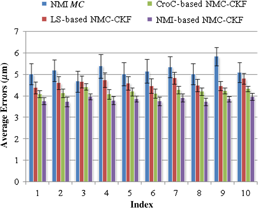
We did not use CKF filtering in the first three sets of experiments, where the goal was to evaluate the performance of CKF filtering coupled with different image similarity measures. Figure 4 plots the motion estimation errors calculated between the reference frames and the consequent frames (after motion correction) for one simulated image series. It can be seen that the overall performance using CKF filtering is better than those that did not use it, and as for different image similarity measures, NMI outperformed others. This may be because NMI reflects relatively global information, while the other two methods are vulnerable to image variability among different frames. These results confirmed that more accurate motion compensation can be obtained using NMC-CKF. Notice that the periodical changes of the errors shown in Fig. 4 may be caused by the simulated low-frequency respiratory motion (with a period of 3.11 seconds or frequency of 0.32 Hz) and the high-frequency modulation (period of 1.07 s or frequency of 0.94 Hz).

Fig. 4

Comparison of motion compensation errors using different methods for simulated microendoscopy sequences.

More experiments were carried out to test the robustness of the algorithms with respect to the image noises. For this purpose, we changed the standard deviation (STD) of Gaussian noises in the simulated images from 0.08 to 0.13. Figure 5 shows how well the algorithms can tolerate the addition of spatially correlated Gaussian noises to the image intensities. Similar to Fig. 4, we can also conclude that NMC-CKF can obtain more accurate motion compensation of results in different noise levels.

Fig. 5

Average and STD of motion compensation errors for the whole image sequence, with different noise levels.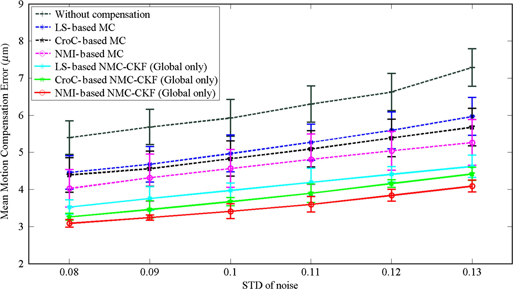

We also used these different similarity measures (i.e., LS, CroC, and NMI) with the NMC-CKF algorithm in the 10 simulated microendoscopy sequences. The error comparison among these three functions is illustrated in Fig. 6, where the STD of noise is 0.12. Same as the experimental results shown in Fig. 4, we did six sets of experiments to determine the best similarity measure. Figure 6 shows the quantitative average transformation errors produced by the NMI-based motion compensation (NMI-based MC) and the NMC-CKF algorithm using three similarity measures. From the previous experimental results, the accuracy using NMI-based MC is better than using LS-based motion compensation (LS-based MC), and CroC-based motion compensation (CroC-based MC). Thus, in Fig. 6, we did not show the results using LS-based MC and CroC-based MC. The experimental results in Fig. 6 show that the NMI-based NMC-CKF method obtained the best accuracy after motion compensation. Figure 7 illustrates an example of the alignment results using NMI-based MC and NMC-CKF, respectively. The difference images are also shown in Fig. 7. In this case, the difference between the reference image and the aligned image after using NMC-CKF is smaller than that of NMI-based MC. In addition, Table 1 summarizes the mean value and STD of average errors for the 10 simulated image sequences, where the STD of noise is 0.12. Even though all the algorithms yielded larger motion compensation errors when the noise level increased, compared to those of the similarity measure-based registration and NMC-CKF algorithm using three similarity measures, NMC-CKF using NMI generated the smallest motion compensation errors.

Fig. 6

Average errors (μm) for the 10 simulated image sequences (STD of noise is 0.12).

Fig. 7

One example result for the simulated data, where the similarity measure is NMI. (a) The current frame before alignment; (b) the result of alignment after using NMI-based registration; (c) the result using NMC-CKF (global only); (d)–(f) are the corresponding differential images between (a)–(c) and the reference frame.

Table 1

The Mean and STD of Average Errors (μm) for the 10 Simulated Image Sequences (STD of noise is 0.12)

	NMI-based motion correction	NMC-CKF(LS-based)	NMC-CKF (CroC-based)	NMC-CKF(NMI-based)
Mean	5.166	4.597	4.204	3.826
STD	0.499	0.287	0.177	0.168

3.3.

Microendoscopy Video Results

Microendoscopy videos collected from six experiments on rabbits were used to test the proposed algorithm. Based on the simulation results, we utilized NMI as the similarity measure in our proposed algorithm. For each video, a scene selection method was first applied to cut it into different video clips so that each video clip is guaranteed to contain the same tumor information, and the only variability within each video clip is caused by motion. Altogether, we used 30 video clips from the experiments to evaluate the performance of the motion compensation algorithms. For each video clip, a frame with the least-squared intensity difference to other frames was selected as the reference frame. Figure 8 shows some results using the NMI-based MC and NMC-CKF (similarity measure is NMI). The second column indicates the current frame before registration, the third column shows the results using NMI-based motion compensation, and the last column provides the result using NMC-CKF (similarity measure is NMI). It can be seen that the proposed NMC-CKF yielded relatively small alignment errors.

Fig. 8

Sample results for real microscopy videos using NMI-based methods. (a) The result using NMI-based motion correction; (b) the NMC-CKF result; (c)–(e) the corresponding differential images of the current frame, (a), and (b) to the reference frame, respectively.

To quantitatively evaluate the motion compensation results, the mean squared intensity differences between each registered frame and the reference frame were calculated. Figure 9(a) plots the results from one video, and Fig. 9(b) shows the mean squared intensity differences of all 30 video clips. From Fig. 9, it can be seen that the mean squared differences before motion compensation is larger than after motion compensation. The mean values of mean squared differences before motion compensation (blue lines in Fig. 9) for all image sequences are from 500 to 700. After using NMI-based motion compensation (green lines in Fig. 9), the mean values of mean squared differences for all image sequences are from 100 to 300. So the mean squared differences are reduced 60% to 80% between the situation without motion compensation and the situation after using NMI-based motion compensation. Then, after the proposed NMC-CKF method was used in these image sequences (red lines in Fig. 9), the mean values of mean squared differences for all image sequences are from 50 to 100. Again, the mean squared differences are reduced 50% to 70% between using NMI-based motion compensation and using NMC-CKF motion compensation. The reduction of standard deviations among these experimental results can also be used to illustrate the advantage of our proposed NMC-CKF method. The average value of standard deviations without motion compensation for all 30 data values is around 200. When the NMI-based motion compensation was used, the average value of standard deviations for all 30 data values is around 100. After using our NMC-CKF method, the average value of standard deviations for all 30 data values is reduced to around 30. From these data, it can be seen that the NMC-CKF method supplies stable and accurate motion compensation results for the molecular image analysis. In conclusion, NMC-CKF significantly improved the image intensity differences after motion compensation for all the videos, while the NMI-based motion compensation yields relatively large errors. These results illustrated the effectiveness of our NMC-CKF approach to aligning the microendoscopy image sequences.

Fig. 9

The improvement of squared intensity differences by NMC-CKF, where the mean squared differences before motion compensation are denoted as blue lines, the values after using NMI-based motion compensation are denoted as green lines, and the mean squared differences after the proposed NMC-CKF method was used in these image sequences are denoted as red lines. (a) An example of the improvement for the mean squared difference using NMC-CKF; and (b) the mean and variance of the mean squared intensity differences for the 30 video clips.

After motion compensation, we can provide relatively stable image sequences for visualizing the fluorescence tumor response. Furthermore, quantitative measures such as sequential image histograms and contrasts between high-intensity tumor and low-intensity normal tissues can also be calculated for tumor detection. Although not a quantitative technique to study fluorescence response across subjects, the contrast between high-intensity spots and low-intensity spots of the same subject plays an important role in determining the cancerous response. Notice that the field of view of the fiber-optic probe is $\sim 500 μ m$ , and it shows only a very small portion of the tissue. On the other hand, respiratory motion and heartbeat can be quite large so that significant changes from one image to the other might happen, and some parts shown in one image might not be present in the other. In fact, motion compensation is valid only when the images contain the same or a large amount of common tissue information. Our premise is that motion compensation in our application will be performed only when the probe is targeted to a desired area and immobilized to capture the microscopy images. Therefore, we limit the motion compensation to the image sequences with similar scenes. Before performing the algorithm, we cut the video into different clips so that each video clip can be guaranteed to contain the same tumor information, and the only variability within each video clip is caused by respiratory motion.

4. Conclusion

We proposed a novel motion compensation algorithm, NMC-CKF, for microendoscopy imaging to enhance the ability to detect cancer in a minimally invasive, image-guided system. Different from the traditional image registration methods, the temporal transformation in the video is modeled using a nonlinear system to increase stability. Compared to the image registration based on similarity measurement, NMC-CKF obtained more accurate alignment results in simulated microendoscopy image sequences. For real microendoscopy videos collected by the CellVizio system, the results also exhibited better image similarity after motion correction. These results confirmed the advantages of incorporating CKF into serial image alignment when using optical microendoscopy.

In our future work, we will apply NMC-CKF to our molecular imaging diagnosis system for lung cancer and study quantitative methods to differentiate between cancer and normal tissue types. The molecular image analysis component is a crucial function for the future development of such an intervention system. The motion compensation study using NMC-CKF is the prior step of our molecular image analysis. Based on the motion compensation result, we can easily distinguish the tumor-contained frame from the whole image sequence. In addition, we will implement a computerized classification method in order to detect tumor cells automatically in IntegriSense-based optical images, such that the pathological studies can be processed based on the classification results in the future.

Acknowledgments

This work was supported by the CPRIT grant RP100627 and John S Dunn Research Foundation.

References

1.

M. E. Llewellynet al., “Minimally invasive high-speed imaging of sarcomere contractile dynamics in mice and humans,” Nature, 454 (7205), 784 –788 (2008). http://dx.doi.org/10.1038/nature07104 NATUAS 0028-0836 Google Scholar

2.

A. HoltmaatK. Svoboda, “Experience-dependent structural synaptic plasticity in the mammalian brain,” Nat. Rev. Neurosci., 10 (9), 647 –658 (2009). http://dx.doi.org/10.1038/nrn2699 NRNAAN 1471-0048 Google Scholar

3.

A. NimmerjahnE. A. MukamelM. J. Schnitzer, “Motor behavior activates Bergmann glial networks,” Neuron, 62 (3), 400 –412 (2009). http://dx.doi.org/10.1016/j.neuron.2009.03.019 NERNET 0896-6273 Google Scholar

4.

W. Zhonget al., “In vivo high-resolution fluorescence microendoscopy for ovarian cancer detection and treatment monitoring,” Br. J. Cancer, 101 (12), 2015 –2022 (2009). http://dx.doi.org/10.1038/sj.bjc.6605436 BJCAAI 0007-0920 Google Scholar

5.

F. J. HerthR. EberhardtA. Ernst, “The future of bronchoscopy in diagnosing, staging, and treatment of lung cancer,” Respiration, 73 (4), 399 –409 (2006). http://dx.doi.org/10.1159/000093369 RESPBD 0025-7931 Google Scholar

6.

M. SimonI. Simon, “Update in bronchoscopic techniques,” Pneumologia, 59 (1), 53 –56 (2010). Google Scholar

7.

L. YarmusD. Feller-Kopman, “Bronchoscopes of the twenty-first century,” Clin. Chest Med., 31 (1), 19 –27 (2010). http://dx.doi.org/10.1016/j.ccm.2009.11.002 0272-5231 Google Scholar

8.

T. C. HeZ. Xue, “A minimally invasive multimodality image-guided (MIMIG) molecular imaging system for peripheral lung cancer intervention and diagnosis,” in Proc. Inform. Proc. Comput.-Assist. Inter., 102 –112 (2010). Google Scholar

9.

T. Heet al., “A minimally invasive multimodality image-guided (MIMIG) system for peripheral lung cancer intervention and diagnosis,” Comput. Med. Imag. Graph., 36 (5), 345 –355 (2012). http://dx.doi.org/10.1016/j.compmedimag.2012.03.002 CMIGEY 0895-6111 Google Scholar

10.

L. Shan, “VivoTag-S680-conjugated 3-aminomethyl αvβ3 antagonist derivative for fluorescence molecular tomography of tumors,” Molecular Imaging and Contrast Agent Database (MICAD), National Center for Biotechnology Information, National Institutes of Health, Bethesda, Maryland (2004). Google Scholar

11.

A. D. Mehtaet al., “Fiber optic in vivo imaging in the mammalian nervous system,” Curr. Opinion Neurobiol., 14 (5), 617 –628 (2004). http://dx.doi.org/10.1016/j.conb.2004.08.017 COPUEN 0959-4388 Google Scholar

12.

T. Bojicet al., “Monotone signal segments analysis as a novel method of breath detection and breath-to-breath interval analysis in rats,” Resp. Physiol. Neurobiol., 161 (3), 273 –280 (2008). http://dx.doi.org/10.1016/j.resp.2008.03.001 RPNEAV 1569-9048 Google Scholar

13.

A. E. Deanset al., “Mn enhancement and respiratory gating for in utero MRI of the embryonic mouse central nervous system,” Magn. Reson. Med., 59 (6), 1320 –1328 (2008). http://dx.doi.org/10.1002/(ISSN)1522-2594 MRMEEN 0740-3194 Google Scholar

14.

J. Degermanet al., “An automatic system for in vitro cell migration studies,” J. Micro.-Oxford, 233 (1), 178 –191 (2009). http://dx.doi.org/10.1111/jmi.2009.233.issue-1 0022-2720 Google Scholar

15.

D. S. GreenbergJ. N. D. Kerr, “Automated correction of fast motion artifacts for two-photon imaging of awake animals,” J. Neurosci. Meth., 176 (1), 1 –15 (2009). http://dx.doi.org/10.1016/j.jneumeth.2008.08.020 JNMEDT 0165-0270 Google Scholar

16.

T. Vercauterenet al., “Robust mosaicing with correction of motion distortions and tissue deformations for in vivo fibered microscopy,” Med. Image Anal., 10 (5), 673 –692 (2006). http://dx.doi.org/10.1016/j.media.2006.06.006 1361-8415 Google Scholar

17.

T. Heet al., “A motion correction algorithm for microendoscope video computing in image-guided intervention,” in MIAR 2010 Springer, 267 –275 (2010). Google Scholar

18.

D. A. Dombecket al., “Imaging large-scale neural activity with cellular resolution in awake, mobile mice,” Neuron, 56 (1), 43 –57 (2007). http://dx.doi.org/10.1016/j.neuron.2007.08.003 NERNET 0896-6273 Google Scholar

19.

Y. Huanget al., “Motion compensated fiber-optic confocal microscope based on common-path optical coherence tomography distance sensor,” Opt. Eng., 50 (8), 083201 (2011). http://dx.doi.org/10.1117/1.3610980 0091-3286 Google Scholar

20.

N. Rosenfeldet al., “A fluctuation method to quantify in vivo fluorescence data,” Biophy. J., 91 (2), 759 –766 (2006). http://dx.doi.org/10.1529/biophysj.105.073098 BIOJAU 0006-3495 Google Scholar

21.

P. A. Valdeset al., “Quantitative fluorescence in intracranial tumor: Implications for ALA-induced PpIX as an intraoperative biomarker,” J. Neurosurg., 115 (1), 11 –17 (2011). http://dx.doi.org/10.3171/2011.2.JNS101451 JONSAC 0022-3085 Google Scholar

22.

L. C. G. RogersJ. W. Pitman, “Markov function,” Ann. Probab., 9 (4), 573 –582 (1981). http://dx.doi.org/10.1214/aop/1176994363 APBYAE 0091-1798 Google Scholar

23.

I. ArasaratnamS. Haykin, “Cubature Kalman filters,” IEEE Trans. Automat. Contr., 54 (6), 1254 –1269 (2009). http://dx.doi.org/10.1109/TAC.2009.2019800 IETAA9 0018-9286 Google Scholar

24.

B. K. P. HornB. G. Schunck, “Determining optical flow,” Artif. Intell., 17 (1–3), 185 –203 (1981). http://dx.doi.org/10.1016/0004-3702(81)90024-2 AINTBB 0004-3702 Google Scholar

25.

Y. A. M. Valdiviaet al., “Image-guided fiberoptic molecular imaging in a VX2 rabbit lung tumor model,” J. Vasc. Interv. Radiol., 22 (12), 1758 –1764 (2011). http://dx.doi.org/10.1016/j.jvir.2011.08.025 JVIRE3 1051-0443 Google Scholar

Citation Download Citation

Tiancheng He, Zhong Xue, Miguel Valdivia y Alvarado, Kelvin K. Wong, Weixin Xie, and Stephen T. C. Wong "Nonlinear motion compensation using cubature Kalman filter for in vivo fluorescence microendoscopy in peripheral lung cancer intervention," Journal of Biomedical Optics 18(1), 016008 (7 January 2013). https://doi.org/10.1117/1.JBO.18.1.016008

Published: 7 January 2013

Access the abstract

JOURNAL ARTICLE
11 PAGES

DOWNLOAD PAPER SAVE TO MY LIBRARY

GET CITATION

CITATIONS

Cited by 2 scholarly publications.

Explore citations on Lens.org

RIGHTS & PERMISSIONS

Get copyright permission Get copyright permission on Copyright Marketplace

KEYWORDS

Video

Tumors

Complex systems

Luminescence

Tissues

Filtering (signal processing)

Image registration

1.

Introduction

2.

Methods