2.1.

Specimens and Preparation

Mouse tail tendons were extracted from wild-type Col1a1 mice and fixed in formalin for 24 h and then stored in phosphate buffered saline (PBS) at 4°C. It has been demonstrated that fixation does not alter the underlying fibrillar collagen structure and the resulting SHG properties^36–38 and primarily results in a slight volumetric shrinking.³⁹ For imaging, a single fascicle was pulled from the tail, and a small section was cut lengthwise, placed on a microscope slide with a drop of PBS, and sealed with a coverslip using nail polish (Sinful Colors). The samples varied in diameter from 60 to 90 μm. The thickness for each is estimated from the image data and the averaged $z$-profile intensity. Tendons were acquired from three mice, and three samples were imaged from each. As mouse tendons were too small to adequately fill the area of the laser spot in bulk measurements, rat tail tendons were used instead. Here, two to three rat tail tendons were used, where they were cut and folded out on a microscope slide to extend the width, and a coverglass was put on top to further increase the spread area and to ensure that all the space interacting with the laser was filled.

2.2.

SHG Microscope and Measurements

The SHG microscope and data acquisition protocols have been described elsewhere.⁴⁰ Briefly, a Ti:Sapphire laser is coupled to a homebuilt laser-scanning system (WiscScan) on a fixed stage upright microscope base (Olympus, Center Valley, Pennsylvania BX61WI) microscope. A $40\times 0.8$ numerical aperture (NA) water immersion objective and 0.9 NA condenser are used for excitation and collection, respectively, of the forward SHG signal. The backward SHG is collected in a nondescanned geometry, where the detector is in the infinity space. Both detection channels use Hamamatsu, Hamamatsu, Japan 7422-40P GaAsP photomultiplier tube (PMT)s. The calibration of the efficiencies of the forward and backward detection paths was obtained by two-photon excited fluorescence imaging of beads that emit in the same wavelength range as the detected SHG signal. The laser excitation wavelength range was 890 to 1230 nm and provided by a Coherent Chameleon, Santa Clara, California Ultra Ti:Sapphire oscillator (680 to 1080 nm tunability) and a synchronously pumped APE Optical Parametric Oscillator (1050 to 1700 nm tuning range). For all excitations, the corresponding SHG signal is filtered with 20-nm full width at half maximum bandpass filters (Semrock, Rochester, New York FF01-445/20, FF01-494/20, FF01-583/22, and FF01-615/20). The setup is designed such that both sources have the same beam size entering the microscope and follow the same optical path, allowing robust switching through two high-precision motorized stages. Circularly polarized light, as determined at the focus, is used throughout to avoid alignment specific effects.

The F/B versus depth measurement was made for the entire thickness of the tendon. Each was made in triplicate, where for each specimen the data was obtained sequentially across the wavelength range. The SHG intensities were integrated across the whole tendon. Image analysis was performed using FIJI (an open-source platform for biological-image analysis)⁴¹ and MATLAB.

2.3.

Bulk Optical Property Measurements

We recently described a new approach to bulk optical property measurements used to determine ${\mu }_s$ and $g$.⁴² For fibrillar tissues with little absorption, such as the tendon used here, the overall attenuation can be approximated by ${\mu }_s$ alone, which we obtain through a measurement of the on-axis attenuation of the tissue sample. Goniometry is used to determine the effective scattering anisotropy $g_{\mathrm{eff}}$, which is reduced from the true single-scattering value when the tissue is more than one scattering length in thickness. With independent knowledge of ${\mu }_s$ and tissue thickness, a series of forward Monte Carlo simulations based on MCML³⁵ is used to obtain the best fit for the single-scattering anisotropy. The merged parameter ${\mu }_s^{\prime }$ is then compared with that extracted through the measured SHG F/B versus depth response across the 890- to 1230-nm wavelength range.

2.4.

Simulation Framework

We previously extended²⁵ the MCML framework³⁵ to allow for focusing of light and SHG creation directionality and conversion efficiency, as well as the primary and secondary filters effects on the SHG creation and propagation, respectively. As will be described in detail in Sec. 3.2, we now fit the simulated F/B response to simultaneously extract ${({\mathrm{F}}_{\mathrm{SHG}}/{\mathrm{B}}_{\mathrm{SHG}})}_{\text{creation}}$ values and ${\mu }_s^{\prime }$. The new extended code was first validated in several ways. First, we verified that the modifications did not affect the original photon migration functionality by running several identical simulations that did not use any of the new features. Second, to validate the collection framework, we simulated isotropic fluorescence from within the sample and validated that the collection was as expected from the solid angle of the collection geometry (both forward and backward) in cases where no scattering or absorption was present and the refractive index mismatch of all layers was identical to avoid reflections. Third, to validate that the SHG directionality was modeled correctly, the detected SHG F/B was measured in a nonabsorbing, nonscattering sample with no refractive index mismatch and was verified to be the same as the specified ${({\mathrm{F}}_{\mathrm{SHG}}/{\mathrm{B}}_{\mathrm{SHG}})}_{\text{creation}}$.

In our previous treatment, no collection apertures were included in the modeling. Here, we have modified the simulations to account for the effect of the aperture, as multiply scattered photons can miss collection and result in erroneous F/B ratios. The available apertures in the backward and forward directions are defined by the NA of the objective and condenser lenses, respectively. The geometry used in the simulation is shown in Fig. 1. The simulation framework has a defined sampling width $\mathrm{d}x$, i.e., constant for both the forward and backward geometries. We set $\mathrm{d}x=2D_{\mathrm{B}}\tan {\theta }_{\mathrm{B}}$ and $D_{\mathrm{F}}=\mathrm{d}x/2\tan {\theta }_{\mathrm{F}}$, where $D_{\mathrm{B}}$ and $D_{\mathrm{F}}$ denote the distances from the focus to the backward and forward detectors, respectively, and ${\theta }_{\mathrm{F}}$ and ${\theta }_{\mathrm{B}}$ are the collection angles defined by the condenser and objective for forward and backward SHG, respectively. In practice, the thickness of the sample is very thin compared with $D_{\mathrm{F}}$, minimizing possible alignment artifacts. The Monte Carlo framework software is available upon request.

Fig. 1

Monte Carlo simulation geometry for collection of the second-harmonic generation (SHG) signal, where $D_{\mathrm{B}}$ and $D_{\mathrm{F}}$ denote the distances from the focus to the backward and forward detectors, respectively, and ${\theta }_{\mathrm{F}}$ and ${\theta }_{\mathrm{B}}$ are the collection angles defined by the condenser and objective for forward and backward SHGs, respectively.

3.1.

Effects of Collection Apertures and Optical Parameters on F/B Response

3.1.1.

Effects of aperture size on the collection of forward and backward components

In prior work, we suggested that in tissues of 5 to 10 mean free path lengths for scattering in thickness, multiply scattered photons could be deviated at angles outside the NA of the collection optics.³⁰ Specifically, for the case of excitation becoming more proximal to the forward tissue exit, backward propagating photons would have an increasing probability of not being collected, resulting in an erroneously high F/B ratio. In our previous work,²⁵ we included the NA in the excitation to simulate optical sectioning; however, the respective forward and backward collection apertures were not included. Here, we updated the framework to this geometry and examined the effect on the resulting F/B ratios as a function of tissue thickness. Figure 2(a) shows the simulated F/B over 100 μm with excitation $\mathrm{NA}=0.8$ for 0.5 NA and 100% collection (as was previously assumed in the simulation) assuming typical parameters for tendon at 890 and 445 excitation and SHG emission, respectively,^30,43 where ${\mathrm{F}}_{\mathrm{SHG}}/{\mathrm{B}}_{\mathrm{SHG}}=9$, ${\mu }_s=450{\mathrm{cm}}^{-1}$, ${\mu }_a=10{\mathrm{cm}}^{-1}$, and $g=0.91$. Near the top entrance of the tissue ($z=0$), the differences between the effective apertures are not significant but increase rapidly for excitation at greater depths. Specifically, at 100 μm into the tissue, the simulated F/B is much smaller using complete (and nonphysical) collection relative to that obtained the actual 0.8 NA by almost a factor of 1.5 (7 versus 11) due to missed photons in the backward channel. To further visualize this effect, consider the hypothetical case of 0.5 NA collection, where we observe apparent increasing (and artifactual) F/B near the bottom exit of the tissue as more backward propagating photons fail to become collected within this aperture. Thus, even for a relatively thin tissue of 100 μm of thickness, corresponding to $\sim 2$ mean free path lengths for scattering in tendon, this shows the importance of including the apertures within the simulation framework to accurately extract the emitted creation ratio from the experimental data.

Fig. 2

Effects of collection aperture with 0.8 numerical aperture excitation on the depth-resolved forward/backward (F/B) (a) and backward attenuation (b) responses using previously determined bulk optical property measurements on tendon.

We can also examine the effect of the objective NA on the measured attenuation of the backward-detected SHG as a function of excitation depth into the tissue. This response results from a combination of the square of the primary filter effect at the laser wavelength and the secondary filter effects at ${\lambda }_{\mathrm{SHG}}$. Using the same conditions as in Fig. 2(a) and now including a primary filter effect of ${\mu }_s=250{\mathrm{cm}}^{-1}$, Fig. 2(b) shows the resulting simulations over the same range of collection NAs. Here, assuming 100% collection underestimates, the rate of decay relative to that which would be measured using the 0.8 NA of the excitation/collection objective by approximately two-fold.

3.1.2.

Effect of optical parameters on F/B measurement via Monte Carlo simulation

We now demonstrate the effect of the individual parameters ${({\mathrm{F}}_{\mathrm{SHG}}/{\mathrm{B}}_{\mathrm{SHG}})}_{\text{creation}}$, ${\mu }_s$, ${\mu }_a$, and $g$ on the F/B versus depth response when corrected for the collection apertures. Figure 3(a) illustrates simulated F/B ratios as a function of imaging depth $z$ for increasing ${({\mathrm{F}}_{\mathrm{SHG}}/{\mathrm{B}}_{\mathrm{SHG}})}_{\text{creation}}$ ratios over the range of 1 to 19 with typical ${\mu }_s$, ${\mu }_a$, and $g$ values for the tendon. In the case of ${\mathrm{F}}_{\mathrm{SHG}}/{\mathrm{B}}_{\mathrm{SHG}}=1$, the resulting F/B ratio is $<1$ at the tissue entrance due to scattering and becomes approximately the SHG creation ratio in the mid-region of the tissue. For higher ${({\mathrm{F}}_{\mathrm{SHG}}/{\mathrm{B}}_{\mathrm{SHG}})}_{\text{creation}}$ values, the $\mathrm{F}/\mathrm{B}(z)={({\mathrm{F}}_{\mathrm{SHG}}/{\mathrm{B}}_{\mathrm{SHG}})}_{\text{creation}}$ point is found increasingly toward the bottom of the sample. However, the location cannot be predicted fully analytically and, therefore, we need to utilize the Monte Carlo simulations using the measured bulk optical properties to obtain the ${({\mathrm{F}}_{\mathrm{SHG}}/{\mathrm{B}}_{\mathrm{SHG}})}_{\text{creation}}$ values from the experimental data. Figure 3(b) illustrates the effect of varying only the scattering coefficient ${\mu }_s$ with other parameters fixed at comparable values, as we have previously reported for collagenous tissues. This primarily affects the slope of the resulting curve, with higher scattering coefficients resulting in steeper slopes. Figure 3(c) shows the effect of fixing the other parameters and varying the scattering anisotropy coefficient $g$, where this has a similar effect on strongly affecting the slope of the F/B curve. We have verified that different combinations of ${\mu }_s$ and $g$ yielding the same ${\mu }_s^{\prime }$ gave indistinguishable F/B versus depth curves for the same SHG creation ratio. This was performed for a range of ${\mu }_s^{\prime }$ from 20 to $80{\mathrm{cm}}^{-1}$ with two representative combinations tested for each case (not shown). This verification affords extracting both ${({\mathrm{F}}_{\mathrm{SHG}}/{\mathrm{B}}_{\mathrm{SHG}})}_{\text{creation}}$ and ${\mu }_s^{\prime }$ from the measured F/B without the need for separate bulk optical property measurements (see Sec. 3.2). Figure 3(d) illustrates the effect of varying the absorption coefficient with the other parameters fixed. For collagenous tissues, the absorption is much weaker than scattering in this spectral region, and as a result, the curves in Fig. 3(d) are similar, showing that this parameter does not change the shape of the curve significantly and will be not be further considered in the analysis.

Fig. 3

Effects of the following optical parameters on the depth-resolved F/B ratio through simulations. (a) ${\mathrm{F}}_{\mathrm{SHG}}/{{\mathrm{B}}_{\mathrm{SHG}}}_{\text{creation}}$, ${\mu }_s$, $g$, and ${\mu }_a$. Other parameters were kept fixed as indicated in each figure.

3.2.

Obtaining both ${\mathrm{F}}_{\mathrm{SHG}}/{\mathrm{B}}_{\mathrm{SHG}}$ and ${\mu }_s^{\prime }$ from Fits to Depth-Resolved F/B Data

We next describe the simulation-based procedure of simultaneously obtaining ${({\mathrm{F}}_{\mathrm{SHG}}/{\mathrm{B}}_{\mathrm{SHG}})}_{\text{creation}}$ and ${\mu }_s^{\prime }$ from experimental F/B versus depth data without the need for separate bulk measurements. Figure 4(a) illustrates the process that generates tables of F/B values versus depth curves for a set of input parameters. We simulate ${({\mathrm{F}}_{\mathrm{SHG}}/{\mathrm{B}}_{\mathrm{SHG}})}_{\text{creation}}$ from 1 to 20 in 100 steps and ${\mu }_s^{\prime }$ from 5 to $50{\mathrm{cm}}^{-1}$ in 100 steps, and the F/B ratio is obtained at depths 0 to $d$ in thickness in 30 steps. The simulations were performed on the Center for High Throughput Computing cluster at the University of Wisconsin, Madison. As the tendon samples varied somewhat in thickness, we generated seven separate tables with each thickness between 60 and 90 μm with a 5-μm step size. Figure 4(b) illustrates the data-processing steps required to obtain an experimental curve of F/B ratios, as a function of depth. We note that the process is averaged over the field-of-view after thresholding the image to eliminate background noise.

Fig. 4

Flowcharts illustrating the full process going from data acquisition to obtaining ${({\mathrm{F}}_{\mathrm{SHG}}/{\mathrm{B}}_{\mathrm{SHG}})}_{\text{creation}}$ from fitting to simulations. (a) Generation of forward simulations, (b) loading of experimental data, and (c) fitting experimental to simulated data.

Figure 4(c) shows the full process of fitting the experimental data to the simulated curves to obtain values of ${\mu }_s^{\prime }$ and ${({\mathrm{F}}_{\mathrm{SHG}}/{\mathrm{B}}_{\mathrm{SHG}})}_{\text{creation}}$. This is done by calculating the reduced chi-squared coefficient between every simulated and experimental curve and determining the range of parameters that yield good fits to the experimental data, where the criterion of ${\chi }_{\text{red}}^2\le 1$ is used and is calculated by

In Fig. 5, we show representative fits of the experimental data to simulations at 890-nm excitation to obtain ${({\mathrm{F}}_{\mathrm{SHG}}/{\mathrm{B}}_{\mathrm{SHG}})}_{\text{creation}}$ and ${\mu }_s^{\prime }$. In the simulations shown in Fig. 5(a), ${\mu }_s^{\prime }$ was fixed, and the best fit for ${({\mathrm{F}}_{\mathrm{SHG}}/{\mathrm{B}}_{\mathrm{SHG}})}_{\text{creation}}$ was found for three cases of the former via single-parameter fitting, where the acceptable fitting condition was ${\chi }_{\text{red}}^2\le 1$. Here, good fits were obtained for a range of ${\mu }_s^{\prime }$ between 52 and $106{\mathrm{cm}}^{-1}$, with a best fit at ${\mu }_s^{\prime }=(79\pm 25{\mathrm{cm}}^{-1})$. Analogous fits were performed for a several creation ratios between 5.8 and 6.76 with a range of ${\mu }_s^{\prime }$ values (not shown). The best resulting fit ${({\mathrm{F}}_{\mathrm{SHG}}/{\mathrm{B}}_{\mathrm{SHG}})}_{\text{creation}}$ was $6.3\pm 0.5$ and similar to our previous results. The overall fitting results are shown in Fig. 5(b), where the ${({\mathrm{F}}_{\mathrm{SHG}}/{\mathrm{B}}_{\mathrm{SHG}})}_{\text{creation}}$ and ${\mu }_s^{\prime }$ are plotted with the corresponding ${\chi }_{\text{red}}^2$ values. This shows that for good fits (${\chi }_{\text{red}}^2\le 1$), the acceptable range of ${({\mathrm{F}}_{\mathrm{SHG}}/{\mathrm{B}}_{\mathrm{SHG}})}_{\text{creation}}$ values is much narrower than for ${\mu }_s^{\prime }$. Therefore, we conclude that the method has higher sensitivity to extracting ${({\mathrm{F}}_{\mathrm{SHG}}/{\mathrm{B}}_{\mathrm{SHG}})}_{\text{creation}}$ than for obtaining ${\mu }_s^{\prime }$ values. However, the method does obtain both ${({\mathrm{F}}_{\mathrm{SHG}}/{\mathrm{B}}_{\mathrm{SHG}})}_{\text{creation}}$ and ${\mu }_s^{\prime }$ values with acceptable fits based on the chi-squared criterion. We stress that the uncertainty in the ${\mu }_s^{\prime }$ values does not significantly affect the obtained ${({\mathrm{F}}_{\mathrm{SHG}}/{\mathrm{B}}_{\mathrm{SHG}})}_{\text{creation}}$ values, as all the best fits [Fig. 5(c)] are closely grouped around $\sim 6$ for a wide range of ${\mu }_s^{\prime }$ values (50 to $100{\mathrm{cm}}^{-1}$).

Fig. 5

Single example of fitting to the SHG creation ratio and reduced scattering coefficient for mouse tendon data. (a) Fits to several representative combinations of ${({\mathrm{F}}_{\mathrm{SHG}}/{\mathrm{B}}_{\mathrm{SHG}})}_{\text{creation}}$ and ${\mu }_s^{\prime }$ values with goodness of fit. The resulting best fits were ${({\mathrm{F}}_{\mathrm{SHG}}/{\mathrm{B}}_{\mathrm{SHG}})}_{\text{creation}}=6.3\pm 0.5$ and ${\mu }_s^{\prime }=79\pm 25{\mathrm{cm}}^{-1}$ and (b) goodness of fits to ${({\mathrm{F}}_{\mathrm{SHG}}/{\mathrm{B}}_{\mathrm{SHG}})}_{\text{creation}}$ and ${\mu }_s$. A small range in creation ratios are obtained across a wider range of reduced scattering coefficients.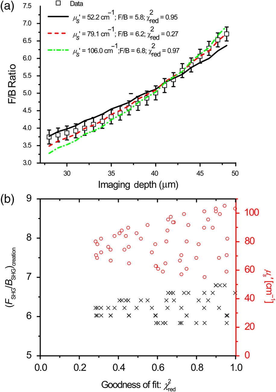

3.3.

Spectral Slope Analysis

Figure 6 shows the dependence of the extracted reduced scattering coefficients from the SHG F/B data [hereafter denoted as ${\mu }_s^{\prime }(\mathrm{SHG})$] over the range of SHG emission wavelength of 445 to 615 nm. This was initially performed for verification of the new analysis by comparison with prior bulk optical property measurements. However, if good agreement is obtained, this may obviate the need for separate bulk measurements for tissues that can be imaged on the SHG microscope. These data were averaged over several tissues, whereas the data and fits in Fig. 5 were the result of a single run. The Shapiro-Wilk test was run to determine if the data were normally distributed and if the Student $t$-test was appropriate for the analysis. This condition was satisfied, and Table 1 lists the $p$ values from pairwise $t$-tests between the results for every combination of wavelengths. With the exception of 535 and 615 nm, the extracted ${\mu }_s^{\prime }(\mathrm{SHG})$ values are statistically different at the $p<0.05$ level. Thus, we conclude that the trend of decreasing ${\mu }_s^{\prime }$ with increasing wavelength was statistically significant.

Fig. 6

Wavelength dependency of (a) ${\mu }_s^{\prime }$ and (b) SHG creation ratio. Dataset for three different samples at three spots in each case. The error bars shown are the standard error of the mean.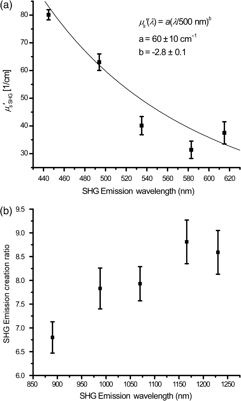

Table 1

Results of pairwise t-tests for the best fits of μs′ data between the different wavelength groups, where p<0.05 values were considered to be statistically different. Only the 535 and 615-nm points were not significantly different.

Table 2 lists the values as obtained by conventional bulk optical property measurements²² (${\mu }_s^{\prime }$) and the fitting procedure from the SHG F/B data [${\mu }_s^{\prime }(\mathrm{SHG})$]. We note that the bulk optical property measurements were done on rat tail tendon rather than mouse tail tendon, as the latter is too small for complete overlap with the $\sim 1\text{-}\mathrm{mm}$ laser spot even when unwrapped and flattened. Moreover, the former is too thick to image in its entirety. However, transmission electron microscopy of both mouse and rat tails suggests that they have a similar distribution in fibril diameters.^44,45 As both SHG and scattering properties are governed by the fibrillar structure, their respective attributes are also expected to be similar. Moreover, the fibrillar structures of these tissues are similar when viewed in the SHG microscope.

Table 2

Comparison of the reduced scattering coefficient as obtained by bulk optical property measurements and retrieved from fits. The uncertainty is the standard deviation.

By comparing the tabulated data, we found that the ${\mu }_s^{\prime }(\mathrm{SHG})$ is roughly a factor of 2.5 times larger than ${\mu }_s^{\prime }$ at the wavelengths listed (with some nonsystematic variations). This indicates that the wavelength dependence of both factors is linearly related by a constant coefficient. We have verified this by fitting the results to the power law ${\mu }_s^{\prime }(\lambda )=a{(\lambda /500\mathrm{nm})}^b$ over the same wavelength range. This best fit showed that the $a$ factor increased by roughly a factor of 2.5 ($80\pm 29$ versus $31.2\pm 9.6{\mathrm{cm}}^{-1}$), whereas the scattering power $b$ was not significantly different ($2.8\pm 0.2$ versus $2.7\pm 0.2$).

We propose two possible reasons for the difference in scattering magnitude extracted by the two methods: (1) the local environment around the SHG creation region has a higher “local” scattering coefficient than the bulk due to dense fibril structure which is required for efficient SHG, which further has a quadratic dependence on concentration, i.e., less dense regions may contribute to the bulk ${\mu }_s^{\prime }$ but not to the SHG signal; and (2) the radiation pattern of SHG emission is not directly on axis in the forward and backward directions, but instead has an angular distribution with a defined “phase function” (emission intensity as function of radiation angle). In this case, a higher number of emission scattering events would be required to emulate the experimental data, which only integrates forward and backward intensities within the NA of the condenser and objective, respectively. Our observations are consistent with either explanation. We note that the somewhat limited number of data points over a fairly broad wavelength range and relatively large uncertainty does not allow for highly accurate power-law fitting. Moreover, the resulting power law dependencies have been shown to depend on the range of wavelengths used for fitting.⁴⁶ However, based on theoretical modeling by Rogers et al.,⁴⁷ the spectral dependence or spectral slope of ${\mu }_s^{\prime }$ carries the structural information related to scatter size and packing, more so than the absolute values. Indeed, the $b$ coefficients reflecting the spectral slope were similar for both methods (2.8 versus 2.7).

Further studies are required to fully analyze and understand the reason for the higher ${\mu }_s^{\prime }(\mathrm{SHG})$ values. Such studies of the precise shape of the radiation pattern might also be of interest for a wide variety of studies and could give more information to the underlying tissue structure rather than just the relative strength of the F/B ratios. We emphasize that the obtained ${\mu }_s^{\prime }(\mathrm{SHG})$ may be useful for differentiating diseased versus normal tissues. For example, our limited data (two wavelengths) comparing ${\mu }_s^{\prime }$ between normal and ovarian cancer showed a marked difference in spectral slope.²⁶ We also extracted marked differences in the SHG creation ratio and have seen large differences in the fibrillar morphology. Thus, it would be advantageous to simultaneously acquire SHG image data and concurrently extract ${({\mathrm{F}}_{\mathrm{SHG}}/{\mathrm{B}}_{\mathrm{SHG}})}_{\text{creation}}$ and the spectral slope of ${\mu }_s^{\prime }$ as a generalized means to classify tissue.

3.4.

Wavelength Dependence of ${({\mathrm{F}}_{\mathrm{SHG}}/{\mathrm{B}}_{\mathrm{SHG}})}_{\text{creation}}$

Figure 6(b) shows the resulting wavelength dependency of the ${({\mathrm{F}}_{\mathrm{SHG}}/{\mathrm{B}}_{\mathrm{SHG}})}_{\text{creation}}$ values for mouse tail tendon samples. The Shapiro-Wilk test showed that the data were normally distributed, and $t$-tests were used here for statistical analysis, as in Sec. 4. Paired $t$-tests between the different groups, listed in Table 3, show that all the measured creation ratios are statistically significantly ($p<0.05$) different with two nonsystematic exceptions. Thus, we conclude that the trend of increasing ${({\mathrm{F}}_{\mathrm{SHG}}/{\mathrm{B}}_{\mathrm{SHG}})}_{\text{creation}}$ values with increasing wavelength was statistically significant.

Table 3

Results of pairwise t-tests for the best fits of (FSHG/BSHG)creation data between the different wavelength groups, where p<0.05 values were considered to be statistically different. Statistically insignificant p values have been marked for clarification.

This increasing ratio is indicative of the phase mismatch $\mathrm{\Delta }k=k_{2\omega }-2k_{\omega }$ decreasing with increasing wavelength. In SHG microscopy, this mismatch is determined by the harmonophore distribution and associated spatial frequencies, the Gouy phase shift, and dispersion between the laser and SHG wavelengths.^21,48 Although the relative contributions of these factors are not yet fully understood, the overall trend is consistent with the reduced dispersion at longer wavelengths, as $\mathrm{\Delta }k$ decreases and the emission becomes more forward directed, i.e., has a longer coherence length.

This finding is in contrast to other papers examining the wavelength dependence of the SHG creation ratio. For example, recently Shen et al.⁴⁹ found no wavelength dependent effects and speculated that the backward signal arose from reflections of forwarded emitted SHG. We believe this is unlikely as completely forward-directed emission would require type I or II phase-matching conditions where $\mathrm{\Delta }k=0$. Such conditions do not exist in collagen. In further contrast, Theodossiou et al.⁵⁰ found differing wavelength dependencies for the forward and backward responses and used quasi-phase matching arguments to explain their findings. We note that these two studies utilized very thin sections of a few microns in thickness. Although the results from such specimens are nominally free of scattering, cutting effects can result in highly spatially dependent densities and be in significant differences in the measured F/B. We have not been able to obtain consistent results from such thin sections, and we posit that more accurate measurements are obtained from intact tissues with proper accounting of the scattering.