Adaptive row-action inverse solver for fast noise-robust three-dimensional reconstructions in bioluminescence tomography: theory and dual-modality optical/computed tomography in vivo studies

Ali Behrooz; Chaincy Kuo; Heng Xu; Brad W. Rice

doi:10.1117/1.JBO.18.7.076010

10 July 2013 Adaptive row-action inverse solver for fast noise-robust three-dimensional reconstructions in bioluminescence tomography: theory and dual-modality optical/computed tomography in vivo studies

Ali Behrooz, Chaincy Kuo, Heng Xu, Brad W. Rice

Author Affiliations +

Journal of Biomedical Optics, Vol. 18, Issue 7, 076010 (July 2013). https://doi.org/10.1117/1.JBO.18.7.076010

Abstract

A novel approach is presented for obtaining fast robust three-dimensional (3-D) reconstructions of bioluminescent reporters buried deep inside animal subjects from multispectral images of surface bioluminescent photon densities. The proposed method iteratively acts upon the equations relating the multispectral data to the luminescent distribution with high computational efficiency to provide robust 3-D reconstructions. Unlike existing algebraic reconstruction techniques, the proposed method is designed to use adaptive projections that iteratively guide the updates to the solution with improved speed and robustness. Contrary to least-squares reconstruction methods, the proposed technique does not require parameter selection or optimization for optimal performance. Additionally, optimized schemes for thresholding, sampling, and ordering of the bioluminescence tomographic data used by the proposed method are presented. The performance of the proposed approach in reconstructing the shape, volume, flux, and depth of luminescent inclusions is evaluated in a multitude of phantom-based and dual-modality in vivo studies in which calibrated sources are implanted in animal subjects and imaged in a dual-modality optical/computed tomography platform. Statistical analysis of the errors in the depth and flux of the reconstructed inclusions and the convergence time of the proposed method is used to demonstrate its unbiased performance, low error variance, and computational efficiency.

1. Introduction

Bioluminescence tomography (BLT) has found extensive applications in preclinical studies, small animal imaging, cancer research, and drug monitoring and discovery as a noninvasive in vivo molecular imaging platform for three-dimensional (3-D) localization and visualization of the distribution and activity of bioluminescent reporters that label physiological and molecular processes of interest deep inside biological tissue.¹^–⁴ Bioluminescence is a process in which light is produced through oxidation of a class of heterocyclic molecules named luciferin in the presence of the enzyme luciferase.⁵ Bioluminescent compounds are used as bioreporters to tag, track, and monitor molecular and biological processes in laboratory animals.¹ Photons emitted from luminescent probes upon administration of luciferin, though weak in intensity,² can be detected and measured (counted) on the surface of the animal using ultrasensitive charged couple device (CCD) cameras or detector arrays. Quantification and depth-resolved localization of deep tissue bioluminescent reporters from these multispectral boundary measurements in small animals constitute a highly ill-conditioned problem and require inverse solvers that effectively overcome the ill-posed nature of the problem. While least-squares 3-D reconstruction algorithms have been developed for BLT,⁶^,⁷ they require proper parameter selection for optimal performance and suffer from slow convergence when solving large-scale problems.

In this work, we present a row-action unbiased iterative adaptive algebraic reconstruction technique (ART) optimized for fast robust 3-D reconstructions in BLT. The proposed method does not rely on optimal parameter selection unlike least-squares methods. The proposed algorithm, named multilevel scheme adaptive algebraic reconstruction technique (MLS-AART), is designed for remarkably fast convergence to unbiased stable solutions and is optimized according to the properties of the data and constraints of bioluminescence imaging. To validate the performance of the proposed method, it is applied to a total of 10 phantom-based and dual-modality optical/computed tomography (CT) in vivo studies, and the errors in the reconstructed volume, depth, and flux intensity along with convergence time of the algorithm are computed and analyzed statistically. The statistical study of error in the 15 reconstructed inclusions shows that the proposed algorithm has an unbiased low-variance performance especially in depth estimation and flux quantification and a remarkably low average convergence time compared to existing row-action inverse solvers.

2. Background

In BLT, multispectral measurements of the diffuse luminescent photons on the animal surface are used for depth-resolved localization and quantification of the 3-D distribution of bioluminescent reporters buried deep in the tissue.⁶ Propagation of emitted luminescent photons in highly scattering low absorptive media such as tissue is modeled by the diffusion equation, expressed in Eq. (1), which is a first-order approximation to the radiative transfer equation and has been shown to accurately model diffuse photon propagation.⁸

Eq. (1)

D \nabla^{2} Φ (r) - μ_{a} Φ (r) = - q (r) .

In Eq. (1), $Φ (r)$ represents average light intensity, $μ_{a}$ is the absorption coefficient, $D$ is the diffusion coefficient, and $q (r)$ is the luminescent source flux at location $r$ . Numerical techniques such as the finite element method are often used to discretize Eq. (1) and numerically solve for its Green’s functions. However, the excessive computational and memory requirements of these techniques make them less efficient compared to faster semianalytical solvers. It has been shown that for a homogeneous medium (medium with spatially uniform absorption and scattering coefficients), a tangential planar approximation can be used to find a semianalytical formulation for the Green’s functions of Eq. (1) as shown below,⁶

Eq. (2)

G_{i j} = \frac{1}{2 π D} [\frac{\exp (- μ_{eff} r_{i j})}{r_{i j}} - \frac{1}{z_{b}} \int_{0}^{\infty} \exp (\frac{- x}{z_{b}}) \frac{\exp [- μ_{eff} \sqrt{{(d_{j} + x)}^{2} + p_{i j}^{2}}]}{\sqrt{{(d_{j} + x)}^{2} + p_{i j}^{2}}} d x],

where

d_{j}

is the distance of the voxel indexed

i

from the tangent plane at the boundary point indexed

j

, and

p_{i j}

is the distance of the boundary point indexed

j

from the point on the plane closest to the voxel indexed

i

and so

r_{i j} = \sqrt{d_{j}^{2} + p_{i j}^{2}}

. The parameters

μ_{eff}

and

z_{b}

depend on the geometry of the medium and its optical properties.⁹

Using Eq. (2), the Green’s function describing the boundary distribution of the photons emanating from an arbitrary point source inside a turbid medium can be obtained analytically. Since the Green’s functions of Eq. (2) are wavelength dependent, multispectral data are acquired to enhance the information content of the measurements and constrain the solution. Using a 3-D grid to discretize the medium and the Green’s functions corresponding to the voxels of the grid, a linear relationship can be established between the flux of the bioluminescent agents at the voxels of the 3-D grid and the boundary measurements of luminescent light intensity as formulated below:

Eq. (3)

ρ = Gs,

where

ρ

is the data vector that lists the multispectral boundary measurements,

s

is the luminescence flux vector, and

G

is the system matrix that depends on the optical properties and the geometry of the turbid medium and whose columns are the discretized Green’s functions for the voxels corresponding to the entries of

s

.

BLT aims at retrieving the luminescence distribution vector $s$ using the measurements $ρ$ and an estimate of the system matrix $G$ . It involves a highly ill-posed inverse problem,¹⁰^,¹¹ as the 3-D depth-resolved map of bioluminescence source flux distribution must be reconstructed from two-dimensional (2-D) boundary measurements. Conventionally, reconstruction algorithms resort to least-squares regularization methods¹⁰^,¹²^–¹⁴ to overcome this ill-posedness. However, in these techniques, optimal selection of the regularization parameter is needed to avoid over- or under-regularization. Also, the computational cost and memory requirements for numerical implementation of some regularization-based reconstruction algorithms are considerably high.¹⁴^,¹⁵Although a priori information can be incorporated into regularization and least-squares methods to enhance stability and numerical efficiency,¹⁶^,¹⁷ they are not always available in bioluminescence imaging studies.

Iterative row-action reconstruction methods¹⁸^,¹⁹ are a class of memory-efficient low-cost numerical solvers that avoid bulky matrix computations in large-scale problems by iteratively updating the solution using only one equation at a time. As a result, these methods only involve one-dimensional vector computations. The most popular iterative row-action methods are ARTs that have recently found extensive applications in medical and molecular image reconstruction.²⁰^–²³ In conventional ART, the solution is updated at each iteration through an orthogonal projection to the hyperplane of the corresponding equation in the linear system of equations. Mathematically, given the system of equations defined in Eq. (3), the solution vector denoted by $s$ is updated at the $k$ ’th iteration, corresponding to the $i$ ’th row of the system of equations as below,¹⁹

Eq. (4)

s^{(k + 1)} = \min {‖ s^{k + 1} - s^{k} ‖}_{2} subject to G_{i :} s^{(k + 1)} = ρ_{i},

where

G_{i :}

denotes the

i

’th row of the matrix

G

, and

ρ_{i}

is the

i

’th entry in the data vector. Solving for

s^{(k + 1)}

while enforcing non-negativity (since

s

represents the non-negative flux of bioluminescence at each voxel) yields¹⁹

Eq. (5)

s^{(k + 1)} = s^{(k)} + \frac{ρ_{i} - G_{i :} s^{(k)}}{G_{i :} G_{i :}^{*}} G_{i :}^{*},

Eq. (6)

s^{(k + 1)} = \max (s^{(k + 1)}, 0) .

Equations (5) and (6) are the core components of non-negative conventional ART. It has been shown that the projection access order (order at which the equations are accessed and used for updating the solution) has an important role in the speed of convergence in ART.²⁴^–²⁶ MLS-ART is a modification to conventional ART where the equations are accessed in an optimal order to ensure speedy convergence.²⁴ The access order of equations is considered to be optimal when hyperplanes corresponding to successive equations are orthogonal to each other or intersect at close-to-perpendicular angles. After the equations are reordered to ensure optimal convergence, they are accessed one by one for iterative projections and this continues until each equation has been accessed $N$ times. Figure 1 provides a geometric insight into the dynamics of ART-type algorithms. Figure 1(a) presents a geometrical interpretation of MLS-ART applied to a 2-D problem. Here, each line represents a hyperplane in the solution space corresponding to one of the equations, and the solution is the intersection of the solid lines. The progress of MLS-ART is represented by dark crossmarks and gray arrow lines. As depicted in Fig. 1(a), the points with crossmarks iteratively progress toward the solution (intersection of the two lines) by orthogonal successive projections onto the two lines.

Fig. 1

Geometric interpretations of ART and MLS-AART: red lines represent the two equations in the 2-D solution space. (a) Gray arrows and dark crossmarks show the convergence of ART. (b) Orange arrows and violet dots show the convergence of MLS-AART to the solution (crossing point of two lines). (c) Convergence of MLS-ART and MLS-AART overlaid.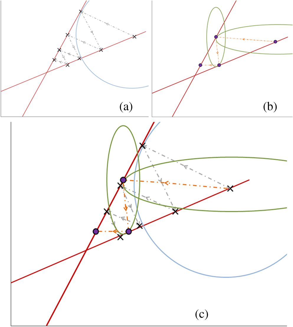

In this paper, we investigate the use of a modified version of MLS-ART that has improved speed and performance over conventional MLS-ART as it smartly guides the projections toward the true solution which increases the speed of convergence and geometric proximity of the result to the true solution.²⁷ The proposed algorithm is called MLS-AART because it adaptively guides the projections to the solution. In Fig. 1(b), the violet dots and orange arrows demonstrate the convergence of MLS-AART algorithm toward the solution. As depicted in Fig. 1(b), in adaptive algebraic reconstruction, the direction of projection at each iteration is inclined toward the crossing point of the two lines making the convergence to the solution faster compared to MLS-ART where the circular (spherical) unit circle of the objective norm results in orthogonal projections. The adaptively inclined projections are a result of the elliptical unit circle of the weighted norm used in MLS-AART. Mathematical details of the proposed algorithm will be discussed in Sec. 3.1.1. In this paper, we optimize and employ MLS-AART for 3-D BLT reconstructions. We validate the performance of MLS-AART using phantom and dual-modality animal studies. The multitude of studies used for validation of the algorithm allows for a statistical study of the mean and standard deviation of the error in the reconstructed volume, depth (defined as the distance along the optical axis of the system from the inclusion to the animal surface facing the camera), and flux of the 3-D bioluminescence distribution as well as the convergence time of the algorithm.

3. Materials and Methods

3.1.

Optimized AART

3.1.1.

General MLS-AART

The MLS-AART can be represented mathematically as follows. In the $k$ ’th iteration of MLS-AART [corresponding to the $i$ ’th row in the linear system of equations expressed in Eq. (3)], the solution is updated as follows:

Eq. (7)

s^{(k + 1)} = \min {‖ s^{k + 1} - s^{k} ‖}_{S^{- 1}} subject to G_{i :} s^{(k + 1)} = ρ_{i},

Eq. (8)

{‖ x^{2} ‖}_{S^{- 1}} = x^{T} diag (\frac{1}{s}) x = x^{T} [\begin{matrix} \frac{1}{s_{1}} & \dots & 0 \\ ⋮ & ⋱ & ⋮ \\ 0 & \dots & \frac{1}{s_{n}} \end{matrix}] x .

Solving for $s^{(k + 1)}$ using Lagrange multipliers²⁸ yields

Eq. (9)

s^{(k + 1)} = s^{(k)} + \frac{ρ_{i} - G_{i :} s^{(k)}}{G_{i :} {SG}_{i :}^{*}} {SG}_{i :}^{*},

Eq. (10)

S = [\begin{matrix} s_{1} & \dots & 0 \\ ⋮ & ⋱ & ⋮ \\ 0 & \dots & s_{n} \end{matrix}] .

MLS-AART, as formulated in Eqs. (9) and (10), must be initialized with a nonzero vector $s^{(0)}$ to converge. To illustrate the dynamics of MLS-AART, we present a 2-D geometrical interpretation as shown in Fig. 1(b). The unit circle of the weighted $L_{2}$ norm denoted by $‖ . ‖_{(S^{(- 1)})}$ is an ellipse in two dimensions and an $n$ -dimensional ellipsoid in higher dimensions with its long diameter lying parallel to the axis corresponding to the largest entry in $s$ . When projections are ordered in a multilevel scheme to maximize orthogonality (or the angle) between successive equations or hyperplanes, the ellipsoid representing the unit circle of the adaptively weighted norm is inclined toward the meeting point of the hyperplanes as shown by the green ellipses in Fig. 1(b). Hence, in each iteration, MLS-AART projects the updates closer to the true solution compared to orthogonal projections as shown in Fig. 1(c), where the progress of MLS-AART and MLS-ART is depicted by orange arrows and violet dots and dark crossmarks and gray arrows, respectively.

3.1.2.

Sampling and ordering of data points

Multispectral noncontact [charge-coupled device (CCD)-based] data acquisition provides a large set of data points ranging from noisy low-intensity to high-intensity data points. High-intensity data provide information about the flux intensity and the coordinates of the source. Low-intensity data, which usually sit on the spatial tails, carry information about the depth and the shape of the inclusion. Additionally, data from lower wavelengths carry more localized information (due to higher tissue absorption) and data from higher wavelengths are more diffuse and less localized. Therefore, finding the optimal sampling strategy which provides the best trade-off between low-intensity and high-intensity data is important for accurate and robust 3-D reconstructions in BLT. In this work, we investigated three sampling distributions on patterns with 200 per wavelength data points: uniform distribution, intensity distribution, and intensity-squared distribution. While for each sampling distribution there are cases for which they work optimally, on aggregate, intensity-weighted sampling resulted in better 3-D reconstructions compared to the uniform and intensity squared.

As discussed in Sec. 2, the optimal projection access order is pivotal to speedy convergence of ART, particularly for MLS-AART.²¹^,²⁴ Ordering the equations to establish maximal independence between successive equations can be done through computing the angle between pairs of hyperplanes representing the linear equations. However, this scheme would be highly time and memory consuming and defeats the purpose of optimizing the proposed algorithm for speedy convergence. Similar to fast projection access ordering schemes used in x-ray CT,²¹ we propose a fast heuristic method for ordering the projections in MLS-AART. After interlacing data points from different wavelengths, equations (data points) are ordered in a fashion that maximizes physical distance between successive data points to ensure minimal correlation between successive equations. Hence, starting from a high intensity point, the algorithm moves to a point farthest from it and then onto a point farthest from both in a max–min fashion and so on. In mathematical terms, at $k$ ’th iteration, the data point $p_{k}$ is picked from

Eq. (11)

p_{k} = {\arg_{p}}_{} \max [\min (dist (p, p_{j})] for \forall j < k,

which is a fast strategy for ordering data points or equations used by MLS-AART. The ordering described in Eq. (11) does not overburden the reconstruction algorithm as its computational complexity for

N

data points is

O (N^{2})

, which, as discussed in Sec. 5, is in the same order as the computational complexity of MLS-AART.

3.1.3.

Non-negativity constraint

Non-negativity in ART is enforced through setting negative entries to zero in the updated solution vector. In MLS-AART, however, zero entries will remain zero since the update equation includes a multiplication by a matrix diagonally populated with the solution vector as formulated in Eqs. (9) and (10). Therefore, setting negative entries to zero cannot be used to enforce non-negativity as the corresponding entry will remain zero for the remainder of the iterations, which will not allow the algorithm to converge to the true solution. Therefore, we use a reflective scheme for non-negativity enforcement. Mathematically, it can be formulated as

Eq. (12)

s^{(k + 1)} = \max (s^{(k + 1)}, - s^{(k + 1)}),

where negative entries are reflected to their positive absolute value. This scheme of non-negativity enforcement does not harm nor limit the convergence of MLS-AART toward the true solution.

3.2.

Multispectral Imaging System

The bioluminescence imaging experiments presented in this paper were conducted using IVIS® Spectrum Imaging System (PerkinElmer, Inc., Alameda, California) that is shown in Fig. 2. The multispectral imaging data collected by IVIS® Spectrum are used for 3-D BLT. This instrument uses a $2048 \times 2048 pixel$ , 26 mm wide, high-sensitivity back-thinned CCD camera for image acquisition while thermoelectrically cooled to $- 90 ° C$ to minimize dark current and other thermal noise effects. The CCD possesses high quantum efficiency ( $> 90 %$ ) over a wavelength range of 400 to 950 nm covering the entire visible and near-infrared range that are of interest in optical imaging. Light is collected and directed to the CCD array using an $F / 1$ aperture lens. The minimum detectable radiance for the system is rated around ${70 photons / s / cm}^{2} / sr$ for integration times up to 300 s allowing for fast collection of weak luminescent signals attenuated by tissue absorption. A filter wheel comprised of 18 custom-designed (transmission $> 95 %$ ) 20-nm band-pass filters spaced every 20 nm from 500 to 840 nm is used in the imaging system.

Fig. 2

Illustration of the IVIS Spectrum imaging system is used for bioluminescence tomography (BLT).

In order to provide consistent measurements in different imaging conditions, the imaging system is calibrated for detection and quantification of very low spectral radiance.²⁹ This calibration provides the conversion of the CCD electron counts to isotropic radiance on the subject surface by taking into account the loss in the optics and the aperture ( $f$ -stop), the field of view (FOV), CCD integration time, binning, and quantum efficiency. The instrument is equipped with a laser and a high-speed scanning galvo mirror system that provides structured illumination for determining the surface topography of the boundary of the small animal being imaged.⁶ The photon density distribution on the surface is calculated from the radiance or counts of the CCD image using the spatial angle between the normal to the surface and the CCD axis as described in Kuo et al.⁶

3.3.

Optical/CT Dual-Modality Imaging and Coregistration

The dual-modality studies presented in this paper are carried out using the IVIS® Spectrum (optical) and the Quantum® FX (x-ray) imaging platforms. The Quantum® FX system (PerkinElmer, Inc., Alameda, California) is a stand-alone micro-CT system for small animal studies. Implants used for the dual-modality studies are made of materials with x-ray opacity noticeably higher than biological tissue and can be segmented out in the CT reconstructions. The 3-D reconstructions from bioluminescence and micro-CT imaging are coregistered using a scheme that involves a position-encoded pattern in the animal restraining bed used for imaging and transport of the anesthetized animal. In our studies, the typical resolution and dosage of a single CT scan are around 100 μm and 8 mgray, respectively.

4. Experiments and Results

We performed a variety of phantom-based and in vivo studies to assess the performance of the proposed optimized MLS-AART in reconstructing luminescent inclusions. In phantom-based experiments, the optical properties are homogeneous and their precise values are known. As a result, these studies are suitable for exploring how the performance of the proposed technique is affected by errors only arising from experimental settings (detector noise, calibration errors, etc.). Verifiable in vivo studies are also used as a highly effective test bed for the proposed reconstruction algorithm as they include all types of the errors and noise contamination present in bioluminescence studies. We use two categories of in vivo luminescent implant studies: (1) fixed-flux radioluminescent implant studies suitable for flux reconstruction validation and (2) sizeable phosphorescent implant studies suitable for depth, flux, volume, and shape reconstruction of differently shaped inclusions. Altogether, these studies provide a comprehensive and varied pool of datasets that can reveal different aspects of the performance of the proposed MLS-AART.

4.1.

Phantom-Based Studies

We utilize a mouse-shaped phantom, as shown in Fig. 3(a), made of polyurethane material that includes scattering particles and absorbing material to mimic the optical properties of biological tissue.³⁰ The phantom is about 9 cm long, 4 cm wide and 2.2 cm high. The mouse-shaped phantoms have hollow regions of different shapes to house light-emitting objects. To mimic the bioluminescence deep inside small animals, optically charged phosphorescent beads were placed inside the phantoms. The two phantom experiments presented in this work comprise of (1) a phosphorescent rod and (2) a phosphorescent disk placed inside phantoms and imaged by the IVIS® Spectrum. Emission properties, flux calibration, and other details regarding the phosphorescent beads used in our experiments are discussed in detail in the Appendix. As depicted in Fig. 3(b) and 3(c), filtered multispectral images were acquired at wavelengths of 560, 580, 600, 620, and 640 nm at an FOV of 13.4 deg with a binning factor of 8 and average exposure time of $15 s / image$ . The 3-D reconstructions were performed on a 3-D grid with 1 mm³ cubic voxels using the proposed optimized MLS-AART as shown in Fig. 3(b) and 3(c). The 3-D reconstructions visually match the phosphorescent inclusions while errors in reconstructed flux average around 9% and errors in reconstructed depth average around 12% for the phantom studies.

Fig. 3

(a) Mouse-shaped phantom made of polyurethane material with scattering and absorptive pigments to mimic tissue optical properties. This phantom has rod-shaped hollow regions to house light sources of cylindrical shapes. Tissue phantom experimental studies: (b) data from disk-shaped source inside XPM phantom and 3-D reconstruction using MLS-AART. (c) Data from rod-shaped source inside XPM phantom and 3-D reconstruction using MLS-AART.

4.2.

In Vivo Radioluminescent Implant Studies: Quantification Validation

In the first category of the in vivo experiments, calibrated radioluminescent tritium-filled glass beads are implanted surgically at fixed locations in live mice under anesthesia.⁶^,³¹ With a diameter of around 1 mm and a length of 5 mm, the barrel-shaped beads maintain a fixed radiant flux of $3.6 \times 10^{10} photons / s$ .

Four tritium bead experiments are presented in this paper for in vivo validation of the proposed MLS-AART as depicted in Fig. 4: (1) two beads implanted 2 mm deep in the pelvic fat region of a nu/nu mouse and imaged on the ventral side, (2) two beads implanted 4.5 and 5.9 mm deep in left and right thighs of a nu/nu mouse, respectively, and imaged on the dorsal side, (3) two beads implanted 4 mm deep in the left and right thighs of a nu/nu mouse and imaged on the ventral side, and (4) one tritium bead implanted 3 mm deep in the scruff region of a nu/nu mouse and imaged on the dorsal side. All cases were imaged at wavelengths of 560, 580, 600, 620, and 640 nm at an FOV of 12.6 deg with a binning factor of 8 and average exposure time of $1 s / image$ . Structured light analysis was performed to render the mouse boundary visible to the camera lens. While no a priori information regarding the shape, size, or position of the implants is used by the reconstruction algorithm, the volume over which the reconstruction is performed is limited to the 3-D space laterally bounded by the coordinates of the data points used by the algorithm.

Fig. 4

In vivo studies for flux quantification of radioluminescent implants in nu/nu mice: (a) ventral view data from two tritium beads implanted in pelvic fat region of a nu/nu mouse;(b) reconstruction of the pelvic fat implants using MLS-AART;(c) data fidelity or fit between simulated from reconstructed sources and original data;(d) reconstruction using MLS-AART for dorsal data from two tritium beads implanted in thighs of a nu/nu mouse;(e) reconstruction using MLS-AART for ventral data from two tritium beads implanted in thighs of a nu/nu mouse; and (f) reconstruction for dorsal data from a tritium bead implanted in the scruff region of a nu/nu mouse.

3-D reconstructions are performed for the four in vivo experiments described above on a 3-D grid with 1 mm³ cubic voxels using MLS-AART as shown in Fig. 4. The reconstructed inclusions are small in size and have spherical or cylindrical shapes as expected. The error in the reconstructed depth averages around $- 6 %$ , and the error in the reconstructed flux averages around 3.5% for these studies. Hence, there is good agreement between the tritium bead shapes, flux, and depth and the corresponding reconstructions. In Fig. 4(c), the fit between the measured data and the simulated data from the reconstruction in Fig. 4(b) is shown. Despite the presence of optical heterogeneities in the organs of the nu/nu mouse imaged in this experiment, the data simulated from the reconstructed sources match the measured data very well. The good data fit further demonstrates the validity of the homogeneous model used in this work.

4.3.

In Vivo Phosphorescent Implant Studies: X-Ray CT Validation

While tritium beads are useful models of in vivo point sources, they do not allow for validation of shape reconstruction in a more extended geometry. To accomplish this, we use sizeable phosphorescent beads of various shapes implanted at different depths in live nu/nu mice. The phosphorescent material employed in the implants is copper-doped zinc sulfide ( $ZnS : Cu$ ), which is used extensively in glow-in-the-dark paint.³² $ZnS : Cu$ phosphorescence emission, which is the result of optically excited electrons decaying between Cu impurity states, has a relatively slow decay and hence a long life-time which makes it particularly attractive to our in vivo implant studies. Meanwhile, $ZnS : Cu$ has higher x-ray opacity compared to the organs and soft tissue surrounding it when implanted in small animals. Therefore, these implants provide high contrast in x-ray CT imaging, allowing them to be localized in the 3-D CT image. The CT map of the $ZnS : Cu$ inclusions is used as a reference for validation of the 3-D bioluminescence reconstructions. Depth and volume of $ZnS : Cu$ implants are obtained from the 3-D CT images. The reconstructed $ZnS : Cu$ maps from x-ray CT are coregistered with the 3-D reconstructions from optical imaging for visual assessment. The $ZnS : Cu$ beads used in the implant studies, their flux decay, and their emission spectrum curves are depicted in Fig. 5. Details regarding the calibration of the flux of the $ZnS : Cu$ implants are described in the Appendix.

Fig. 5

Phosphorescent copper-doped zinc sulfide beads made as in vivo implants: (a) elbow shaped, (b) disk shaped of different sizes, and (c) ring shaped. (d) Blue curve (circles) shows the decay of phosphorescent emission intensity versus time for a $ZnS : Cu$ bead. Green curve (plus-signs) shows the inverse square root of the same emission intensity versus time which has a linear behavior. (e) Emission spectrum of $ZnS : Cu$ peaks around 540 nm.

After optical imaging is performed, the anesthetized mouse is directly transported to and scanned by the x-ray CT system where a 3-D CT map of the phosphorescent implant is obtained. Four $ZnS : Cu$ in vivo studies, as shown in Figs. 6 and 7, are performed: (1) a sizeable $ZnS : Cu$ ring, about 6 mm in diameter, is implanted 4 mm deep in the intestines of a nu/nu mouse and imaged at 580, 600, 620, 640, 660 nm and also scanned by the CT system as depicted in Fig. 6(a) and 6(b); (2) a sizeable $ZnS : Cu$ disk is implanted 4 mm deep in the intestines of a nu/nu mouse whose CT map is depicted in Fig. 7(a); (3) two $ZnS : Cu$ cylinders are implanted 4 mm deep and 6 mm apart in the intestines of a nu/nu mouse whose CT map is depicted in Fig. 7(d); and (4) a $ZnS : Cu$ cylinder and a ZnS:Cu elbow are implanted 5.6 and 5.1 mm deep in the left and right thighs of a nu/nu mouse, respectively, whose CT map is depicted in Fig. 7(g). For all cases, the imaging is performed with an FOV of 13 deg, a binning factor of 8, and average exposure time of $3 s / image$ .

Fig. 6

In vivo dual-modality optical/CT imaging experiment with a $ZnS : Cu$ phosphorescent ring implanted in the intestines of a nu/nu mouse.(a) Ventral view data from the ring-shaped $ZnS : Cu$ implant in the intestines of the nu/nu mouse. (b) X-ray CT 3-D map of the mouse with ring-shaped $ZnS : Cu$ implant. (c) BLT 3-D reconstruction for ring-shaped implant. (d) Coregistered overlaid bioluminescence and CT reconstruction for ring-shaped implant. (e) Data fit between the acquired data and simulated data from reconstructed sources for ring-shaped implant.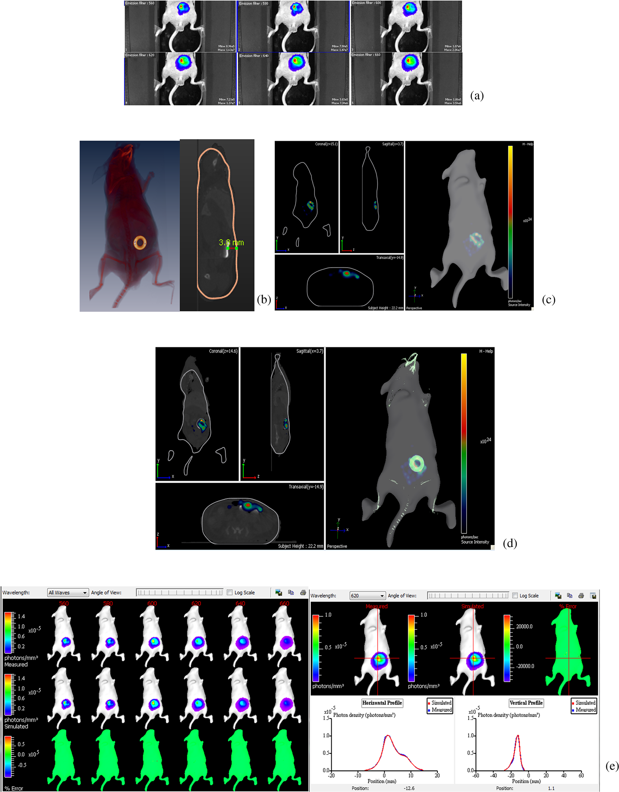

Fig. 7

Three in vivo studies with CT validation of $ZnS : Cu$ phosphorescent implants in nu/nu mice.(a) X-ray CT 3-D map of disk-shaped $ZnS : Cu$ implant. (b) BLT 3-D reconstruction of the disk-shaped implant. (c) Coregistered overlaid bioluminescence and CT reconstruction for disk-shaped implant. (d) X-ray CT 3-D map of cylinder-shaped $ZnS : Cu$ implants. (e) BLT 3-D reconstruction of the cylinder-shaped implants. (f) Coregistered overlaid bioluminescence and CT reconstruction for cylinder-shaped implants. (g) X-ray CT 3-D map of elbow-shaped and cylinder-shaped $ZnS : Cu$ implants. (h) BLT 3-D reconstruction of the elbow-shaped and cylinder-shaped implants. (i) Coregistered overlaid bioluminescence and CT reconstruction for elbow-shaped and cylinder-shaped implants.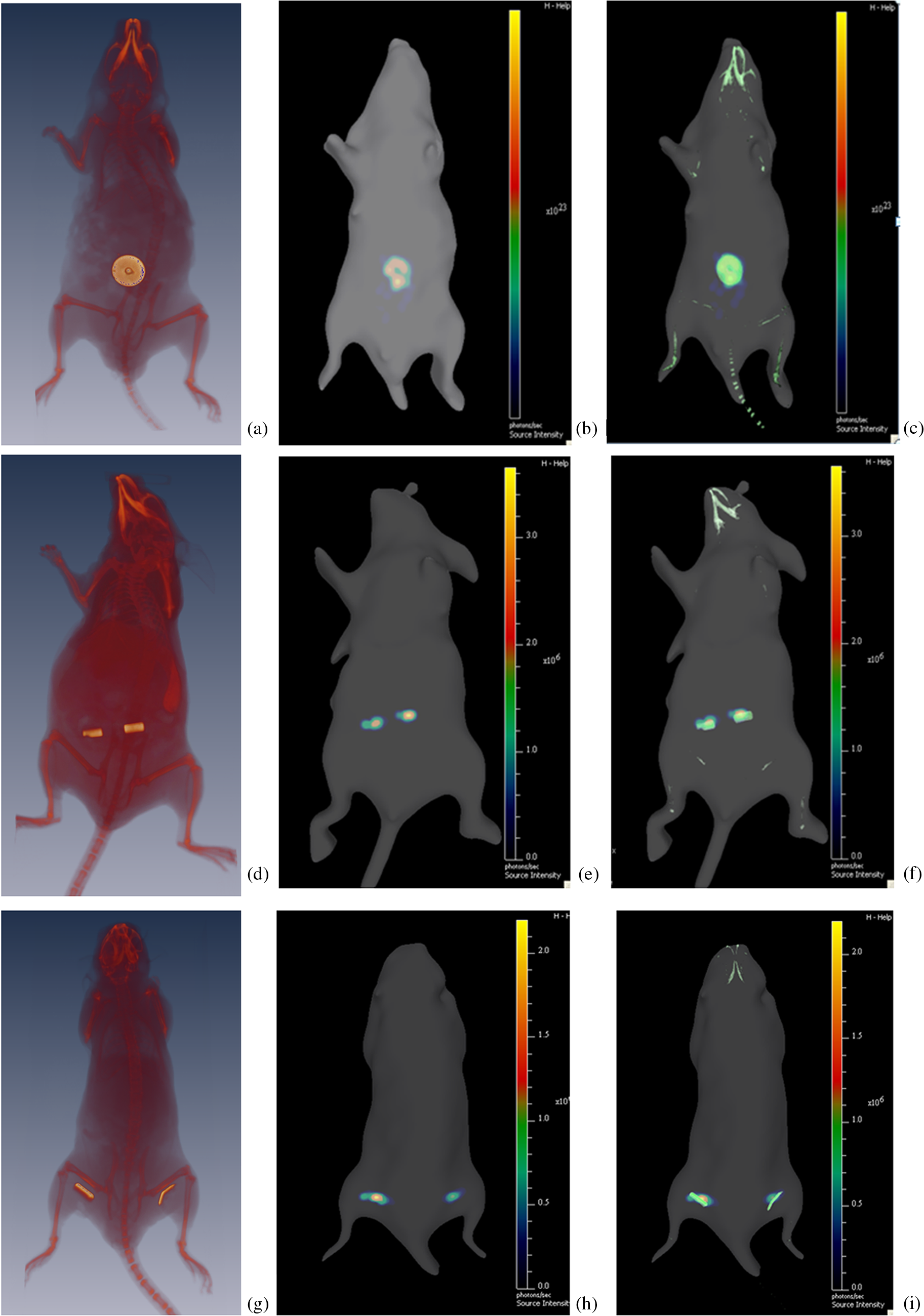

Three-dimensional reconstructions of the $ZnS : Cu$ implant beads from bioluminescence imaging are performed on a 3-D grid with ${1 mm}^{3}$ cubic voxels using MLS-AART as depicted in Figs. 6(c), 7(b), 7(e), and 7(h). Also the coregistered overlaid optical/CT reconstructions are depicted in Figs. 6(d), 7(c), 7(f), and 7(i). As shown in Figs. 6 and 7, the reconstructed inclusions match the shape of the implants visually. The reconstructed depth and flux for the $ZnS : Cu$ experiments have an average error of only 1.2% and 3%, respectively, which further validate the robustness and unbiased nature of MLS-AART reconstructions. Also, as depicted in Fig. 6(e), there is a good fit between the measured and simulated data for the ring-shaped implant study that illustrates the validity of approximations used for optical properties in this work.

5. Discussion and Conclusions

Reconstruction algorithms are an integral part of BLT systems and are required to obtain quantitative source location, size, and flux. Considering the ill-posed nature of the BLT inverse problem, the accuracy and computational efficiency of these algorithms present significant challenges. These algorithms must be robust against errors and noise to achieve stable performance. Techniques such as regularization methods add robustness to reconstruction algorithms by limiting the solution space. This can limit the optimal performance of the algorithms to certain scenarios that make up only a subset of the solution space. Robust yet unbiased algorithms are advantageous to biased algorithms as their performance has the same level of accuracy for all BLT scenarios. Furthermore, the speed of convergence and memory efficiency of reconstruction algorithms must be optimized to avoid excessive computational complexity. MLS-AART is a fast robust unbiased row-action numerical solver that brings all of the desired characteristics together. In this paper, MLS-AART was applied to 3-D reconstruction in BLT. The algorithm relies upon iterative projections onto hyperplanes of the linear system of equations relating the bioluminescence distribution to the data. MLS-AART is memory efficient and fast because it only acts on one equation at a time and processes vectors and diagonal matrices. For a system of equations with $N$ columns (voxels) and $M$ rows (data points), the computational complexity of MLS-AART is O(MN) which theoretically outperforms least-squares based methods.³³ Also, unlike regularization-based methods, MLS-AART is unbiased in nature as it does not favor solutions of certain forms. In a well-posed problem, MLS-AART would converge to the minimum-norm least-squares solution.

The accuracy of reconstructions of luminescent inclusions can be best assessed quantitatively based on the accuracy of depth estimation, flux quantification, and volume reconstruction. Since bioluminescent imaging applications and scenarios are varied in many aspects, a multitude of verifiable studies are required for a thorough statistical analysis of the performance of a reconstruction algorithm. In this work, we presented a total of 10 verifiable BLT studies and experiments that included 15 luminescent inclusions and implants. Therefore, a total of 15 data points are available in this work for statistical study of the error in depth, flux, and volume reconstruction by MLS-AART. The errors associated with MLS-AART reconstructions are summarized in the scatter plots of Fig. 8. The total average error in flux quantification by MLS-AART for the presented studies and experiments is 1.6% with a standard deviation of 18% as represented in Fig. 8(a). The average errors in flux quantification for phantom and in vivo studies are $- 9.5 %$ and 3.3% with standard deviations of 2% and 19%, respectively. The considerably low mean and relatively low standard deviation in flux quantification error demonstrate that statistically, as predicted by theory,¹⁸^,¹⁹^,²⁶ MLS-AART has a low-biased to unbiased performance with a reasonably low error variance. The average error in depth estimation by MLS-AART and the corresponding standard deviation are $- 2.3 %$ and 21.4%, respectively. For the phantom-based and in vivo studies, the average errors in depth estimation are 8.5% and $- 4 %$ with standard deviations of 17% and 22%, respectively. The flux quantification and depth estimation errors are plotted in Fig. 8(a); the red plus signs represent the phantom-based studies, and the blue crossmarks represent the in vivo studies. By visual inspection of Fig. 8(a), the unbiased distribution of the flux and depth errors is evident. Unlike regularized (Bayesian) techniques, where noticeable bias exists in reported results such as in Feng et al.³⁴ in reconstructed flux and depth (reconstructed inclusions are consistently deeper and possess higher flux compared to actual), the reconstruction errors from MLS-AART are quantitatively spread around zero with both positive and negative values. Also, as expected, the standard deviation of the depth and flux error is higher in in vivo studies compared to phantom-based studies. In phantoms, the homogeneous model is valid and the optical properties are known unlike in vivo studies. Nevertheless, the small relative increase in the standard deviation of the error from phantom to in vivo studies shows the robustness of MLS-AART against errors with from by tissue properties’ mismatch and heterogeneities.

Fig. 8

(a) Scatter plot of reconstructed depth and flux error for 15 bioluminescent inclusions in numerical and experimental studies. (b) Scatter plot of reconstructed volume error and convergence time of MLS-AART algorithm for the numerical and experimental studies. (c) Bar plot of MLS-AART convergence time and ART convergence time for the phantom and animal studies.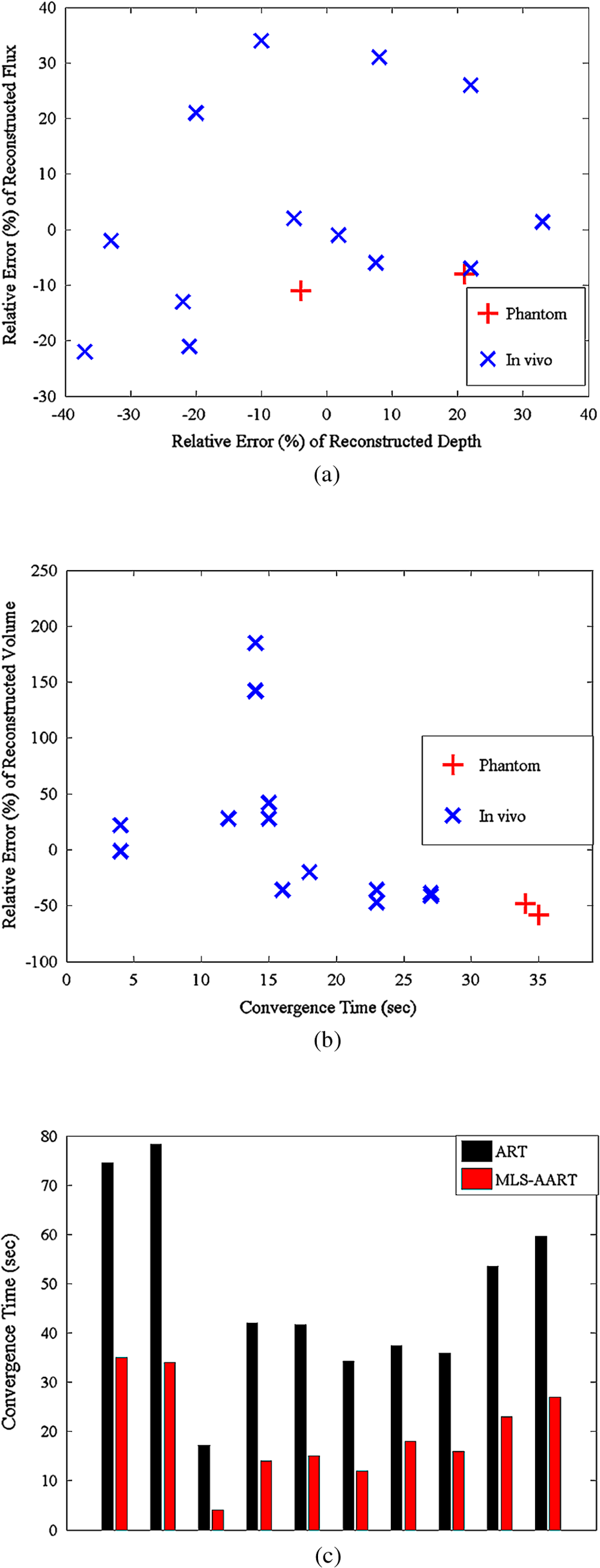

While accuracy in depth and flux and visual match are the most important metrics for assessing the quality of 3-D reconstructions in BLT, we also study the error in reconstructed volume to add a quantitative aspect to the performance of the algorithm in reconstructing the shape and geometry of the inclusions. The average error in volume reconstruction by MLS-AART is around 21% with a standard deviation of 70%. The reconstructed volume errors are summarized in Fig. 8(b). The volume reconstruction errors are higher compared to flux and depth, as inaccuracies in the reconstructed volume are also due to the removal of voxels with low flux values in the reconstructed solutions as well as the discretization of the volume with a 3-D grid.

Moreover, the required times for matrix/vector creation, ordering, and sampling of data, and convergence of the MLS-AART algorithm to the solution for each study, all implemented in C++ on a dual-core processor machine, are plotted in Fig. 8(b). The average required time is 19 s with double-inclusion studies having longer convergence times than single-inclusion studies. When conventional ART was applied to the presented studies, it took an average of 47 s to converge. Figure 8(c) provides a comparison between approximate convergence times of MLS-AART and ART for the presented studies. In our studies, ART required, on average, more than double the time used by MLS-AART to converge to reasonable solutions, especially in studies with sizeable multiple inclusion.

In summary, the statistical study of error in 3-D reconstructions from optimized MLS-AART indicates that the proposed algorithm has an unbiased behavior and a low error variance. Similar to minimum variance unbiased estimators in estimation theory,³⁵ the unbiased and low-variance nature of MLS-AART makes it particularly useful for 3-D reconstructions in imaging modalities with highly ill-conditioned inverse problems. As presented in this work, MLS-AART overcomes the ill-posed nature of the BLT problem, provides robust 3-D reconstructions without limiting the solution space, and ensures stability in the solution without jeopardizing its accuracy. It was also shown to be more computationally efficient and faster than conventional ART.

In conclusion, we presented an optimized non-negative MLS-AART algorithm suitable for 3-D reconstructions from multispectral bioluminescence imaging data. The unbiased low-variance performance of MLS-AART and its speedy convergence were successfully demonstrated using statistical analysis of error and convergence time in 15 reconstructed inclusions from phantom-based and in vivo studies on various parts of mouse body.

Appendices

Appendix

In order to make the $ZnS : Cu$ phosphorescent implant beads, powder-form $ZnS : Cu$ is mixed uniformly with epoxy hardener and resin, and the mixture is poured into polyurethane molds. The epoxy $ZnS : Cu$ mixture completely hardens after 24 h and assumes the shape of its mold. Phosphorescent beads of various shapes, as depicted in Fig. 5(a)–5(c), were made with this procedure. Once optically charged, the beads emit a green glow whose power decays slowly. The decay of $ZnS : Cu$ phosphorescence emission intensity $I (t)$ is best approximated as below:³²^,³⁶

Eq. (13)

I (t) = \frac{I_{0}}{{(1 + kt)}^{2}},

where

k

represents a constant, and

I_{0}

is the initial intensity after charging is completed. The accuracy of Eq. (13) in describing the decay of the phosphorescent implants is pivotal to the precision of flux calibration in the

ZnS : Cu

implant in vivo studies. To examine the accuracy of Eq. (13), we tracked the flux emitted by the

ZnS : Cu

beads using IVIS® Spectrum flux quantification capabilities. The blue curve in Fig. 5(d) represents the measured flux intensity values. From Eq. (13), it follows that the inverse square root of intensity is linear in time as below:

Eq. (14)

\frac{1}{\sqrt{I (t)}} = \frac{1}{\sqrt{I_{0}}} + \sqrt{k} t .

Therefore, the inverse square root of the measured flux intensities should increase linearly with time. The nearly linear green curve in Fig. 5(d) represents the inverse square root of the measured intensity. The linearity of this curve demonstrates the validity of Eq. (14) and hence Eq. (13) in modeling the phosphorescent decay of the $ZnS : Cu$ beads. Therefore using the model formulated in Eq. (13), once the initial flux intensity $I_{0}$ of a charged-to-saturation $ZnS : Cu$ bead is known, the value of its flux intensity can be calculated at later times as long as it receives no optical excitation. The emission spectrum of $ZnS : Cu$ peaks around 540 nm as depicted in Fig. 5(e), whereas the excitation peak lies around 400 nm. For this reason, our experiments show that near-infrared light has no or negligible charging effect on $ZnS : Cu$ beads.

Acknowledgments

The authors would like to thank Dr. Daniel Stearns for his profound contributions to the algorithm development and implant studies presented in this work. The authors also like to acknowledge Ed Lim and Qing Feng for their generous help with in vivo experiments and implementation of algorithms in C++.

References

1.

P. R. Contag, “Whole-animal cellular and molecular imaging to accelerate drug development,” Drug Discov. Today, 7 (10), 555 –562 (2002). http://dx.doi.org/10.1016/S1359-6446(02)02268-7 DDTOFS 1359-6446 Google Scholar

2.

B. W. RiceM. D. CableM. B. Nelson, “In vivo imaging of light-emitting probes,” J. Biomed. Opt., 6 (4), 432 –440 (2001). http://dx.doi.org/10.1117/1.1413210 JBOPFO 1083-3668 Google Scholar

3.

R. WeisslederU. Mahmood, “Molecular imaging,” Radiology, 219 (2), 316 –333 (2001). RADLAX 0033-8419 Google Scholar

4.

V. Ntziachristoset al., “Looking and listening to light: the evolution of whole-body photonic imaging,” Nat. Biotech., 23 (3), 313 –320 (2005). http://dx.doi.org/10.1038/nbt1074 NABIF9 1087-0156 Google Scholar

5.

L. F. Greer IIIA. A. Szalay, “Imaging of light emission from the expression of luciferases in living cells and organisms: a review,” Luminescence, 17 (1), 43 –74 (2002). http://dx.doi.org/10.1002/(ISSN)1522-7243 JLUMA8 0022-2313 Google Scholar

6.

C. Kuoet al., “Three-dimensional reconstruction of in vivo bioluminescent sources based on multispectral imaging,” J. Biomed. Opt., 12 (2), 24007 (2007). http://dx.doi.org/10.1117/1.2717898 JBOPFO 1083-3668 Google Scholar

7.

A. D. Kloseet al., “In vivo bioluminescence tomography with a blocking-off finite-difference SP3 method and MRI/CT coregistration,” Med. Phys., 37 (1), 329 –338 (2010). http://dx.doi.org/10.1118/1.3273034 MPHYA6 0094-2405 Google Scholar

8.

A. Ishimaru, Wave Propagation and Scattering in Random Media, Academic Press, New York (1978). Google Scholar

9.

R. C. Haskellet al., “Boundary conditions for the diffusion equation in radiative transfer,” J. Opt. Soc. Am. A, 11 (10), 2727 –2741 (1994). http://dx.doi.org/10.1364/JOSAA.11.002727 JOAOD6 0740-3232 Google Scholar

10.

P. C. Hansen, Rank-Deficient and Discrete Ill-Posed Problems: Numerical Aspects of Linear Inversion, SIAM, Philadelphia (1997). Google Scholar

11.

G. WangY. LiM. Jiang, “Uniqueness theorems in bioluminescence tomography,” Med. Phys., 31 (8), 2289 –2299 (2004). http://dx.doi.org/10.1118/1.1766420 MPHYA6 0094-2405 Google Scholar

12.

M. Jianget al., “Image reconstruction for bioluminescence tomography from partial measurement,” Opt. Express, 15 (18), 11095 –11116 (2007). http://dx.doi.org/10.1364/OE.15.011095 OPEXFF 1094-4087 Google Scholar

13.

S. Ahnet al., “Fast iterative image reconstruction methods for fully 3D multispectral bioluminescence tomography,” Phys. Med. Biol., 53 (14), 3921 –3942 (2008). http://dx.doi.org/10.1088/0031-9155/53/14/013 PHMBA7 0031-9155 Google Scholar

14.

H. GaoH. Zhao, “Multilevel bioluminescence tomography based on radiative transfer equation part 1: L1 regularization,” Opt. Express, 18 (3), 1854 –1871 (2010). http://dx.doi.org/10.1364/OE.18.001854 OPEXFF 1094-4087 Google Scholar

15.

H. GaoH. Zhao, “Multilevel bioluminescence tomography-based on radiative transfer equation part 2: total variation and l1 data fidelity,” Opt. Express, 18 (3), 2894 –2912 (2010). http://dx.doi.org/10.1364/OE.18.001854 OPEXFF 1094-4087 Google Scholar

16.

W. Conget al., “Practical reconstruction method for bioluminescence tomography,” Opt. Express, 13 (18), 6756 –6771 (2005). http://dx.doi.org/10.1364/OPEX.13.006756 OPEXFF 1094-4087 Google Scholar

17.

J. Fenget al., “An optimal permissible source region strategy for multispectral bioluminescence tomography,” Opt. Express, 16 (18), 15640 –15654 (2008). http://dx.doi.org/10.1364/OE.16.015640 OPEXFF 1094-4087 Google Scholar

18.

A. B. BakushinskyM. Y. Kokurin, Iterative Methods for Approximate Solutions of Inverse Problems, Springer, Dordrecht (2004). Google Scholar

19.

G. T. Herman, Fundamentals of Computerized Tomography: Image Reconstruction from Projections, 2nd ed.Springer-VerlagLondon,2009). Google Scholar

20.

R. GordonR. BenderG. T. Herman, “Algebraic reconstruction techniques (ART) for three-dimensional electron microscopy and x-ray photography,” J.Theor. Biol., 29 (3), 471 –481 (1970). http://dx.doi.org/10.1016/0022-5193(70)90109-8 JTBIAP 0022-5193 Google Scholar

21.

G. T. HermanL. Meyer, “Algebraic reconstruction techniques can be made computationally efficient,” IEEE Trans. Med. Imag., 12 (3), 600 –609 (1993). http://dx.doi.org/10.1109/42.241889 ITMID4 0278-0062 Google Scholar

22.

A. H. Andersen, “Algebraic reconstruction in CT from limited views,” IEEE Trans. Med. Imag., 8 (1), 50 –55 (1989). http://dx.doi.org/10.1109/42.20361 ITMID4 0278-0062 Google Scholar

23.

N. Deliolaniset al., “Free-space fluorescence molecular tomography utilizing 360° geometry projections,” Opt. Lett., 32 (4), 382 –384 (2007). http://dx.doi.org/10.1364/OL.32.000382 OPLEDP 0146-9592 Google Scholar

24.

H. GuanR. Gordon, “A projection access order for speedy convergence of ART (algebraic reconstruction technique): a multilevel scheme for computed tomography,” Phys. Med. Biol., 39 (11), 2005 –2022 (1994). http://dx.doi.org/10.1088/0031-9155/39/11/013 PHMBA7 0031-9155 Google Scholar

25.

X. Inteset al., “Projection access order in algebraic reconstruction technique for diffuse optical tomography,” Phys. Med. Biol., 47 (1), N1 –N10 (2002). http://dx.doi.org/10.1088/0031-9155/47/1/401 PHMBA7 0031-9155 Google Scholar

26.

T. StrohmerR. Vershynin, “A randomized Kaczmarz algorithm with exponential convergence,” J. Fourier Anal. Appl., 15 (2), 262 –278 (2009). http://dx.doi.org/10.1007/s00041-008-9030-4 1069-5869 Google Scholar

27.

L. WenkaiF. F. Yin, “Adaptive algebraic reconstruction technique,” Med. Phys., 31 (12), 3222 –3230 (2004). http://dx.doi.org/10.1118/1.1812606 MPHYA6 0094-2405 Google Scholar

28.

D. P. Bertsekas, Nonlinear Programming, 2nd ed.Athena Scientific, Belmont, Massachusetts (1999). Google Scholar

29.

T. Troyet al., “Quantitative comparison of the sensitivity of detection of fluorescent and bioluminescent reporters in animal models,” Mol. Imag., 3 (1), 9 –23 (2004). http://dx.doi.org/10.1162/153535004773861688 MIOMBP 1535-3508 Google Scholar

30.

M. L. Vernonet al., “Fabrication and characterization of a solid polyurethane phantom for optical imaging through scattering media,” J. Appl. Opt., 38 (19), 4247 –4251 (1999). http://dx.doi.org/10.1364/AO.38.004247 JOAOF8 1464-4258 Google Scholar

31.

M. Fowleret al., “Assessment of pancreatic islet mass after islet transplantation using in vivo bioluminescence imaging,” Transplantation, 79 (7), 768 –776 (2005). http://dx.doi.org/10.1097/01.TP.0000152798.03204.5C TRPLAU 0041-1337 Google Scholar

32.

G. C. LisenskyM. N. PatelM. L. Reich, “Experiments with glow-in-the-dark toys: kinetics of doped ZnS phosphorescence,” J. Chem. Educ., 73 (11), 1048 (1996). http://dx.doi.org/10.1021/ed073p1048 JCEDA8 0021-9584 Google Scholar

33.

A. Bjorck, Numerical Methods for Least Squares Problems, SIAM, Philadelphia (1996). Google Scholar

34.

J. Fenget al., “Three-dimensional bioluminescence tomography based on Bayesian approach,” Opt. Express, 17 (19), 16834 –16848 (2009). http://dx.doi.org/10.1364/OE.17.016834 OPEXFF 1094-4087 Google Scholar

35.

S. M. Kay, Fundamentals of Statistical Signal Processing: Estimation Theory, Prentice-Hall, New Jersey, Englewood Cliffs (1993). Google Scholar

36.

W. H. Byler, “Studies on phosphorescent zinc sulfide,” J. Am. Chem. Soc., 60 (3), 632 –639 (1938). http://dx.doi.org/10.1021/ja01270a040 JACSAT 0002-7863 Google Scholar

Citation Download Citation

Ali Behrooz, Chaincy Kuo, Heng Xu, and Brad W. Rice "Adaptive row-action inverse solver for fast noise-robust three-dimensional reconstructions in bioluminescence tomography: theory and dual-modality optical/computed tomography in vivo studies," Journal of Biomedical Optics 18(7), 076010 (10 July 2013). https://doi.org/10.1117/1.JBO.18.7.076010

Published: 10 July 2013

Access the abstract

JOURNAL ARTICLE
14 PAGES

DOWNLOAD PAPER SAVE TO MY LIBRARY

GET CITATION

CITATIONS

Cited by 15 scholarly publications.

Explore citations on Lens.org

RIGHTS & PERMISSIONS

Get copyright permission Get copyright permission on Copyright Marketplace

KEYWORDS

Reconstruction algorithms

Zinc

Copper

In vivo imaging

Bioluminescence

Error analysis

3D image processing

1.

Introduction

2.

Background

Eq. (1)

Eq. (2)

Eq. (3)

Eq. (4)

Eq. (5)

Eq. (6)

Fig. 1

3.

Materials and Methods

3.1.

Optimized AART

3.1.1.

General MLS-AART

Eq. (7)

Eq. (8)

Eq. (9)

Eq. (10)

3.1.2.

Sampling and ordering of data points

Eq. (11)

3.1.3.

Non-negativity constraint

Eq. (12)

3.2.

Multispectral Imaging System

Fig. 2

3.3.

Optical/CT Dual-Modality Imaging and Coregistration

4.

Experiments and Results

4.1.

Phantom-Based Studies

Fig. 3

4.2.

In Vivo Radioluminescent Implant Studies: Quantification Validation

Fig. 4

4.3.

In Vivo Phosphorescent Implant Studies: X-Ray CT Validation

Fig. 5

Fig. 6

Fig. 7

5.

Discussion and Conclusions

Fig. 8

Appendices

Appendix

Eq. (13)

Eq. (14)

Acknowledgments

References

Show All Keywords

Keywords/Phrases

Search In:

Publication Years