
|
|
1.IntroductionUnveiling fiber map and connectivity patterns in the nervous system are important both in basic neuroscience research and in clinical diagnosis. It is believed now that many brain diseases are associated with abnormity in the white matter.1,2 Diffusion magnetic resonance imaging (dMRI)3 technique provides a unique solution to noninvasively map the white matter in living human brain. Advances in dMRI, such as high-resolution diffusion tensor imaging (DTI),4 high angular resolution diffusion imaging (HARDI),5 or diffusion spectrum imaging (DSI),6 enable investigations at spatial resolutions around 1 mm and with over one hundred directions. Clinical applications have indicated changes in white matter organization in patients with traumatic and ischemic brain injuries and brain tumor, and abnormal connectivity patterns are accompanied by volume change of gray matter in patients with autism or schizophrenia.7,8 Based on those observations, it is reasonable to hypothesize that the alterations in fiber orientations would be a sensitive indicator of brain conditions. However, comprehensive studies on fiber orientations in normal and diseased brains need to be conducted at multiscale resolutions. Light microscopy on histological sections allows single fiber visualization. By using texture analysis on digital images, fiber orientations can be quantitatively assessed. Budde et al.9 applied a Fourier transform algorithm to obtain fiber orientation maps in normal and tumor-induced rat brains. Choe et al.10 used a filter matching algorithm to compare the fiber orientations computed from light microscopy images with dMRI. Wang et al.11 used the gradients of local features on a histology image to quantify the cardiac fiber orientation and validated the measurement of a Jones matrix optical coherence tomography (OCT) technique. The majority of the studies have been performed on two-dimensional (2-D) space, restricted to a small spatial coverage of the tissue, or generating a region of interest (ROI)-based orientation estimation. Global explorations of fiber orientation maps at a microscopic level remain largely unsolved and thus leave a gap with the system-level investigations. OCT12 is a three-dimensional (3-D) imaging technique that enables the visualization of the nerve fiber architecture at micrometer scale resolution.13–15 We have recently reported a serial optical coherence scanner (SOCS) that integrated a vibratome slicer into a multicontrast (MC) OCT system to realize large-scale imaging of ex vivo brain.16 SOCS distinguishes the gray and white matters, provides brain-wide anatomical delineation of fiber architectures, and quantifies the 2-D in-plane (-plane) fiber orientation with intrinsic optical contrasts. However, direct measurement of fiber orientation in the third dimension (with respect to the -axis) is not supported by the current imaging procedure. As a result, efforts in computational analysis may help to recover the inclination angle to complete the orientation information in 3-D space. In this paper, we use the structure tensor (ST) model on SOCS images of ex vivo rat brain to construct quantitative fiber orientation maps in 2-D and 3-D spaces. The ST is typically used to extract features on digital images or volumetric data. It takes the neighboring gradients of a pixel into account and describes the anisotropy and directionality of local textures.17 The approach has been widely used in image or video processing for edge detection and motion tracking.18,19 Biomedical applications of ST include quantitative analysis of anisotropic elements such as collagen networks,20 myocardial fibers,21 and human brain cortex.22,23 Budde and Frank24 applied ST on histological slices of rat brain to examine the fiber orientation in 2-D. Our work demonstrates the use of ST analysis for OCT images and extends previous studies to interrogate 3-D fiber orientations. The ST-based fiber orientation mapping in rat brain is compared with the optic measures of SOCS on the -plane. Because of the analogy of ST with the tensor matrices in DTI, software tools that have been developed for dMRI techniques are readily applicable for visualization, tractography, and connectivity analysis. 2.Materials and Methods2.1.TissueTwo euthanized adult rats were obtained from the tissue sharing program of Research Animal Resources at the University of Minnesota. Brains were dissected and fixed with 10% buffered formalin for 72 h before imaging. 2.2.Serial Optical Coherence Scanner ImagingThe imaging system and associated experimental procedures have been described in detail by Wang et al.16 In brief, SOCS integrates an MC OCT and a microtome slicer to accomplish the reconstruction of macroscopic tissues. Built on a polarization-maintaining-fiber-based polarization-sensitive OCT in the spectral domain,25 the MC-OCT characterizes anisotropic tissues by the optical property of birefringence and incorporates the Doppler flow information when applicable. The light source, a superluminescent diode operating at 840-nm central wavelength with a 50-nm bandwidth, yields an axial resolution of in tissue (with a refractive index of ). The lateral resolution determined by a scan lens () is about . Interference of the backscattered/reflected light from the sample and reference arms is detected by a home-built spectrometer that simultaneously acquires spectra on two orthogonal polarization states. Inverse Fourier transform of the spectral oscillations in -space yields complex-valued depth profiles (A-line) for each polarization channel, which can be represented in polar form as , where and denote the amplitude and phase, respectively, along depth , and the subscripts 1 and 2 correspond to the cross-coupled and main polarization channels. The contrasts for ex vivo brain imaging were generated from the amplitude and phase of the complex-valued depth profiles. These include reflectivity , cross-polarization , retardance , and optic axis orientation . The optic axis orientation, however, is a relative measurement, bearing a time-variant offset that needs to be removed. The offset originates from an arbitrary delay between the optical paths of the two PMF channels. To obtain the absolute optic axis orientation, a retarder film was included as a calibrating reference and imaged together with the tissue. Construction and operation details of the imaging system can be found in our previous publications.16,25 The brain sample was mounted on a vibratome slicer positioned under the scanner. A volumetric scan (optical section) contains 300 cross-sectional frames (B-line) with 1000 A-lines in each frame, covering a field of view of () with a corresponding voxel size of . After imaging one optical section, a superficial slice is removed allowing deeper regions to be imaged. The procedure is repeated until the whole sample is imaged. As the tissue is kept unmoved during the imaging procedures, 3-D reconstruction of the entire sample is achieved by stacking the slices without requiring complicated registration algorithms.16 Two rat brains were scanned, one sectioned in sagittal planes (shown in Figs. 2Fig. 3–4, 6, and 7) and the other in coronal planes (shown in Fig. 5). The sagittal sections consist of 28 slices of 200 μm each, and the coronal sections consist of 66 slices. 2.3.Image ReconstructionThe 2-D en-face images unveil surface and subsurface features within a section. The volumetric datasets of reflectivity, retardance, and optic axis orientation contrasts were projected onto the -plane for each optical section. The pixel intensities in en-face reflectivity and retardance images were computed by taking the corresponding mean value along the depth () direction. The pixel intensities in en-face orientation images were determined by the peak of a histogram formed by binning the measured orientation values along the depth into 2 deg intervals. The depth range used in calculations matches the physical slice thickness. 3-D images of the entire sample block were reconstructed in two ways: by stacking the 2-D en-face images or by stitching the volumetric datasets of all sections. The en-face stack facilitates the global structure identification at a mesoscopic resolution (, the resolution in -axis is constrained by the slice thickness). On the other hand, stitching the volumetric datasets preserves the microscopic resolution as recorded (). For optimal fusing outcome, the starting point along the depth was adjustable to match the ending point of the previous section. The cross-polarization images were used for the 3-D stitching, as the contrast describes the nerve fibers and preserves decent signal intensity in deeper regions. The details of the 3-D reconstructions can be found in our previous publication.16 The reflectivity image portrays the anatomical structures including the fiber tracts, and the retardance and cross-polarization images particularly probe the nerve fibers. They are used as an original dataset to apply ST. The optic axis orientation contrast provides quantification of the in-plane orientation of nerve fibers; therefore, it is used to compare with the results of the ST analysis. Details of the comparison methods are described in the following sections. 2.4.Structure Tensor AnalysisThe ST is a second-moment matrix, which is computed from the gradients of the image data.26 It describes the dominant direction in a local neighborhood of a specific point. The computations are performed based on a pixelwise method.20,24 The procedures are described as follows:
Noise, especially speckle, is a nontrivial problem in coherent and low-coherent imaging systems. Because the speckle pattern in SOCS images can be sensitively captured by the ST analysis, its removal by appropriate filtering is important. We used a nonlinear anisotropic diffusion filter described by Kroon and Slump.27 The filter was applied as a preprocessing step on the original SOCS images. The effectiveness of filtering is evaluated in Sec. 3. The ST algorithms were implemented in MATLAB using customized codes. 2.5.Comparison of Computed and Measured OrientationsThe 2-D computational orientation maps are compared with the en-face optic axis orientation images obtained by SOCS. The orientation differences in selected ROIs are inspected. Since the inclination angle is not measured optically, the comparison of computational and measured orientations is not directly available for 3-D. Instead, we projected the computed 3-D vector onto the -plane and created an en-face image for each optical section using a histogram analysis, as described in Sec. 2.3. The 2-D images derived from the 3-D ST analysis are then compared with the en-face optic axis orientation images. 2.6.TractographySince the ST matrix has the same construction as the tensor data in DTI, tractography tools used for the dMRI technique are readily applicable. We conducted tractography on the 3-D ST data using the Diffusion Toolkit.28 As the tracts are created based on the eigenvectors with respect to the greatest eigenvalues, while in ST the fiber orientation is represented by the vector corresponding to the smallest eigenvalue, we replaced the eigenvalues () with and rebuilt the ST matrix. We demonstrated the results with the interpolated streamline algorithm,29 while application of the fiber assignment by continuous tracking method,30 the second-order Runge Kutta29 and the tensorline31 algorithms showed similar pathways. The tracts are visualized in TrackVis.28 For detailed inspection, ROIs are selected and fibers passing through the nodes are examined. The pipeline of the entire processing is shown in Fig. 1. Fig. 1Processing pipeline of structure tensor (ST) analysis of serial optical coherence scanner (SOCS) images. The optical contrasts are generated for each volumetric scan. En-face images of reflectivity (R) and retardance () are calculated for two-dimensional (2-D) ST computation. Stacked en-face retardance images and stitched optical sections of the cross-polarization (C) contrast are utilized for three-dimensional (3-D) ST computation. The computed orientation maps are obtained through eigen-decomposition of ST and validated by the en-face optic axis orientation images. Tractography is conducted based on the 3-D ST.  3.Results3.1.En-Face Representations of Structure TensorWe applied ST on various contrasts of en-face images. A nonlinear diffusion filter was applied as a preprocessing step on the original images before the ST computation, and the pixel size was interpolated to be . The results with the reflectivity and retardance images are shown in Fig. 2. The left column shows the original images. The reflectivity image is the traditional OCT measure describing the gross structure, but the white matter can be either brighter or darker than the gray matter depending on the fiber orientation with respect to the illumination beam. The retardance image is generated from polarization-sensitive measurement and especially targets the white matter where the birefringence property of myelinated fibers alters the polarization state. The right column shows the computed fiber orientation maps. The images share the same color-coding given on the color wheel, while the brightness is determined by the original SOCS images (left). The results indicate that the computed orientations of the fiber tracts are consistent between the two contrasts. The best agreements are found in regions where fiber identifications are highlighted on both contrasts indicating in-plane alignment of those fiber bundles (e.g., the labeled fiber groups around the medial part of the thalamus). Some discrepancies are observed in the fiber clusters caudal to the thalamus, attributed by the different characteristics revealed on the original images. The result also suggests that the ST analysis can be applied to the images of conventional OCT where the polarization information is not available. As the retardance contrast provides the most robust identification of the white matter on the en-face images,14,17 we apply the 2-D ST on this contrast for further evaluation and comparison. Fig. 2The 2-D ST analysis on (a) en-face reflectivity and (b) retardance images. Left: original images, right: orientation maps computed by eigenvector of ST. Color wheel shows the orientations. Brightness is controlled by the pixel intensities in corresponding en-face images. sm: stria medullaris thalamus, f: fornix, mt: mammillothalamic tract, and fr: fasciculus retroflexus. The round area in blue indicates the ROI 4 for Fig. 4(b). 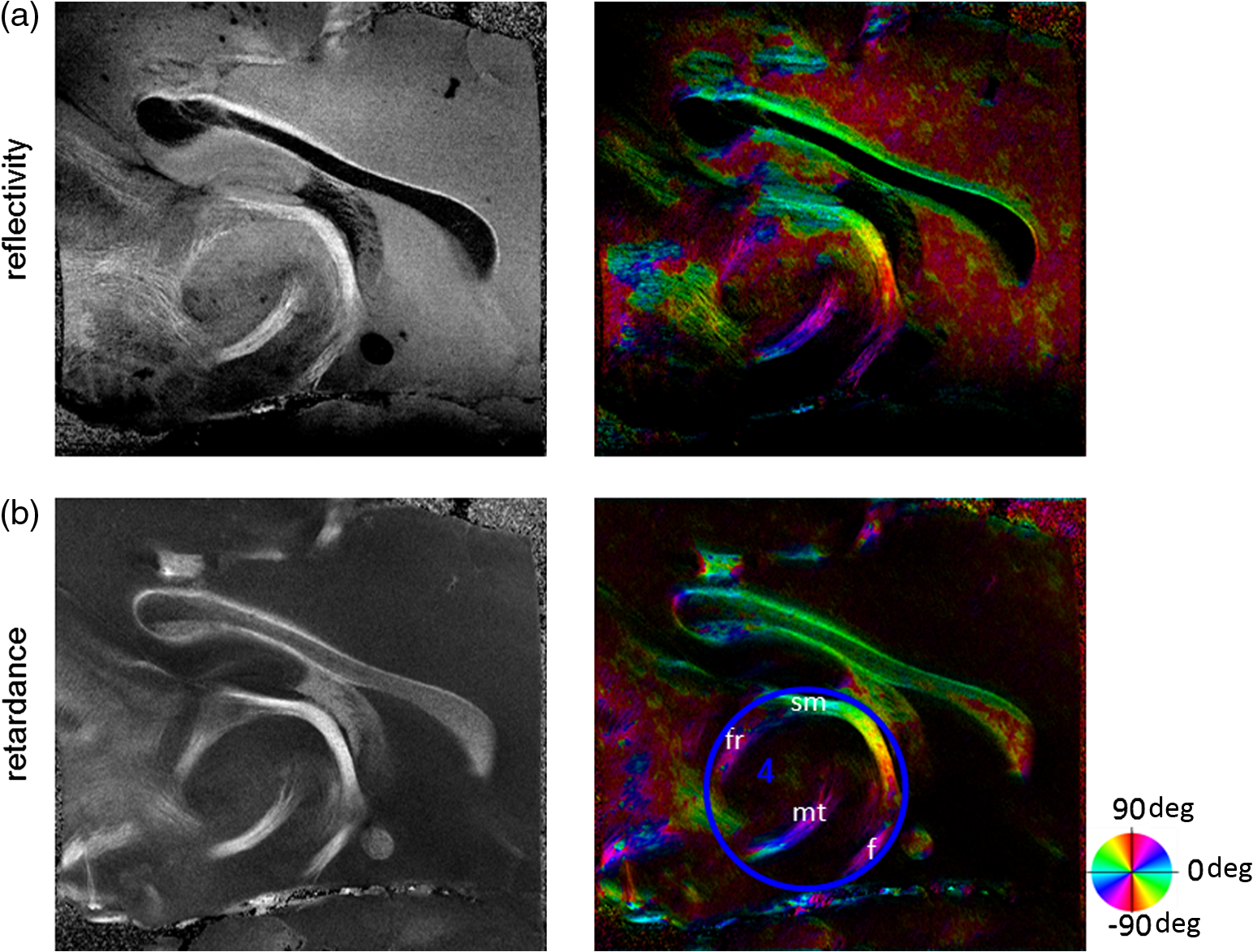 ST is sensitive to abrupt changes in image intensity; as a result, noise reduction plays an important role in obtaining smooth and accurate representations of fiber orientations. Therefore, we applied a nonlinear diffusion filter before ST computation and compared the results with those without any filtering (Fig. 3). Two sizes of smooth kernels, and , were used for the tensor matrices. denotes a Gaussian kernel with the first subscript being the number of neighboring pixels () included and the second subscript being the standard deviation of the Gaussian kernel. The maps are accompanied by the histograms of fiber orientations in an ROI (dashed box). The ROI is placed in the optic tract where coherent orientation is expected in the fiber bundles. When no filter was utilized on the original image, the orientation map is hardly immune from noise (top left) for a smoothing size of (), and the histogram presents a scattered orientation distribution in the optic tract. Increasing the size of the smooth kernel and the weight of the neighboring points enhances the consistency of orientation representation (right column), but results in degraded resolution and misidentification of small crossing fibers if existing. To minimize the problem, a preprocessing step with a nonlinear diffusion filter dramatically reduces the noise while keeping the spatial resolution less affected. We empirically determined to use a smoothing kernel size of 30 to with the preprocessing filter in the following sections. Fig. 3Filtering and kernel size effects on the computational orientation maps: (a) without filter; and (b) with nonlinear diffusion filter applied on SOCS images. The sizes of the smoothing kernels are (left) and (right), respectively, where the first subscript is the number of neighboring pixels included in smoothing and the second subscript is the standard deviation of the Gaussian kernel. The color-coding is in Fig. 2. The white boxes indicate the region of interest (ROI), whose fiber orientation distributions are plotted with histogram (white bars) on individual images (range: , binning: 2 deg).  3.2.Comparison with Optical MeasurementTo evaluate the 2-D ST performance, we compared the computational orientations with the optic axis orientation measurements. Figure 4(a) shows a sagittal slice of the computed and measured orientation maps. The orientation values share the same color coding given by the color wheel. The brightness of the pixels is controlled by the en-face retardance values. The orientation maps demonstrate a remarkable agreement with less than a 10 deg difference in well delineated fibers where higher brightness (retardance) is usually seen. These areas include the internal capsule (ic), the stria medullaris thalamus (sm), the cingulum (cg), and the fiber tracts in the caudate putamen (CPu). More deviations are observed in the white matter regions with low brightness. Fig. 4Comparison of computed and measured orientations: (a) The orientation maps of a sagittal section share the same color-coding (color wheel), and the brightness is controlled by the en-face retardance values. CPu: caudate putamen, TH: thalamus, cc: corpus callosum, and ic: internal capsule. (b) Mean (circles) and standard deviation (bars) of the difference between computed and measured fiber orientations are plotted for all ROIs and respective slices. Pixels having low retardance () are excluded in the statistical analysis. ROIs of the first three plots are indicated on (a). ROI of the last plot contains multiple fiber bundles as shown in Fig. 2 including f, fr, mt, and sm. The ROIs are across multiple slices [-axis in (b)]. 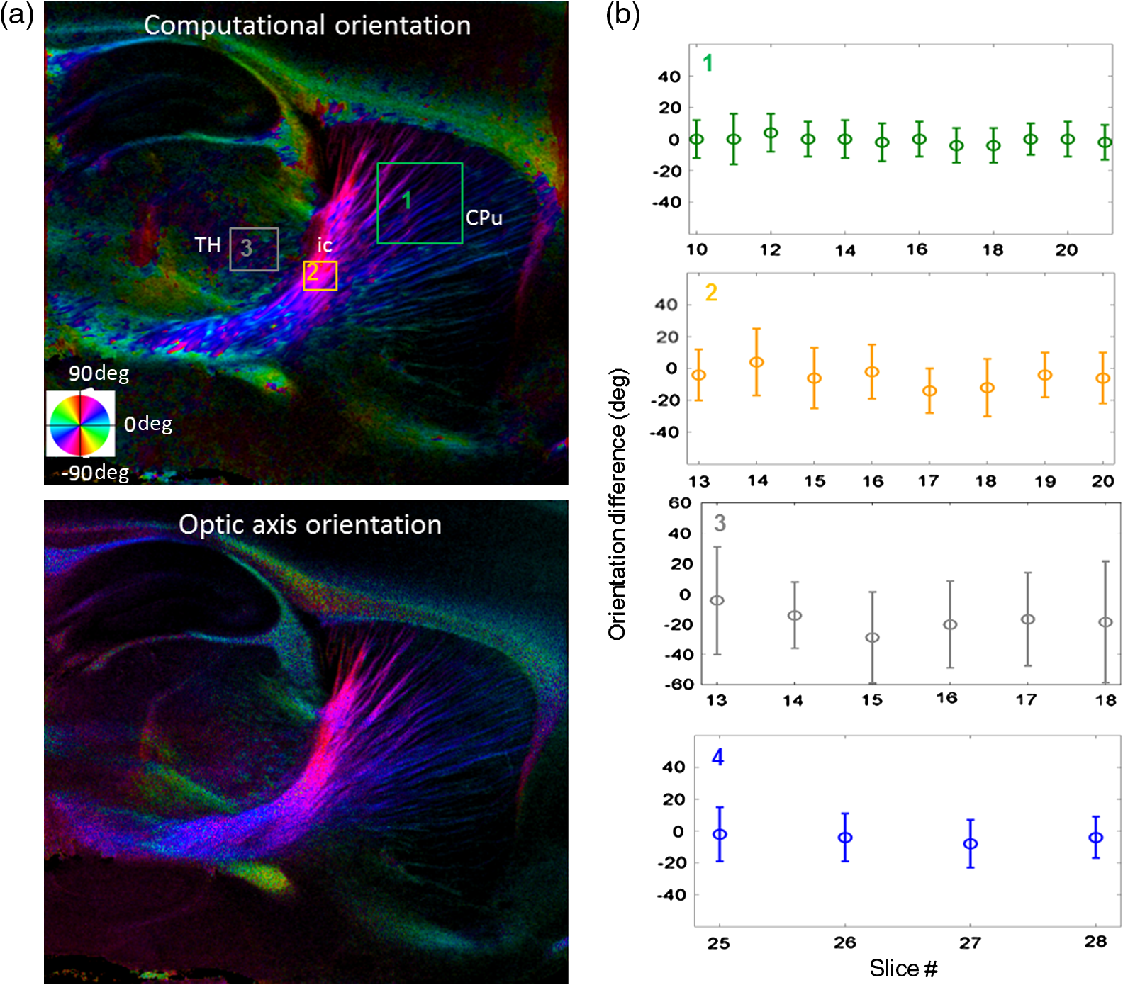 We then performed quantitative comparisons in specific areas of the white matter [Fig. 4(b)]. The ROIs 1, 2, 3 [indicated by the boxes on Fig. 4(a)] contain small fiber tracts in the CPu, dense fiber tracts in the ic, and fiber tracts in the lateral thalamus, respectively. The ROI-4 contains fiber groups around the medial thalamic region including the stria medullaris thalamus (sm), the fornix (f), the mammillothalamic tract (mt), and the fasciculus retroflexus (fr), as indicated in Fig. 2. The ROIs are across multiple slices where the selected architectures are clearly visible. Figure 4(b) shows the plots of mean and standard deviation of the difference between the computed and measured fiber orientations. Pixels having retardance values of 233 nm and higher are included in the statistical analysis. The orientation differences () are , , , and , respectively, for ROIs 1, 2, 3, and 4. The minimal differences indicating good agreement are seen where individual fiber tracts are clearly identified (ROI-1). In addition, the computational orientations are viable in fiber bundles where the dominant features can be captured (ROIs 2 and 4). The orientations are less comparable with greater variations observed in the lateral thalamus (ROI 3) where fiber identification becomes less reliable. 3.3.Three-Dimensional Orientation MapsThe 3-D ST achieves quantification of the fiber orientation in the whole brain space, which fills the gap of current 2-D orientation measurements by SOCS. First, we conducted the ST analysis on the en-face stack of the retardance images. The voxel size of the data was interpolated to be isotropic. This dataset provides a global view of the fiber organization and captures the neural fibers running through the -plane with an inclination angle. Figure 5(a) demonstrates the orthogonal views of the 3-D orientation map derived from the ST. The fiber directions are indicated by the color-coding on each map, and the brightness is controlled by the retardance value. The coronal view (left) shows various fiber groups including the anterior commissure (ac) connecting the two hemispheres in the left-right direction, the f aligned in the superior-inferior direction, and the fibers in the CPu running in the rostral-caudal direction. Color transitions are seen in the fimbria of the hippocampus (fi) and the posterior branch of the anterior commissure (acp). Similar results are seen on the sagittal (middle) and horizontal (right) sections as well. The orientations are consistent with the prior knowledge from dMRI results.32,33 Figure 5(b) demonstrates a microscopic diffusion tensor atlas (resolution: ) of the Wistar rat brain.32 Orthogonal views of 3-D orientation maps are shown at similar locations. The color-coding for orientation is the same as Fig. 5(a). The majority of the fiber orientations obtained by ST are well correlated with the diffusion tensor images. The major deviations in the ST results are observed in the corpus callosum (cc) and external capsule (ec) which form large white matter areas in the absence of the detailed features of fiber bundles. The lack of a dominant direction in local features may induce errors in the orientation estimations within large white matter regions. Fig. 5(a) The 3-D ST for fiber orientations at mesoscopic resolution. The ST is calculated from a stack of en-face retardance images and the orthogonal images are visualized in Vaa3D34 (left: coronal, middle: saggital, and right: horizontal). The color represents the fiber orientations (red: left-right, green: anterior-posterior, and blue: superiorinferior). Directions are labeled on the individual viewing plane. The image intensity is masked by the retardance value which highlights the white matter. CPu: caudate putamen, acp: posterior branch of the anterior commissure, cc: corpus callosum, ec: external capsule, f: fornix, and fi: fimbria of the hippocampus. Sample size: . (b) Microscopic diffusion tensor atlas of a Wistar rat brain (resolution: 50 μm) shows the correspondence with the same color-coding. The fiber orientation maps are shown superimposed on the fractional anisotropy images, which were obtained from the public online dataset at the Duke Center for In Vivo Microscopy. 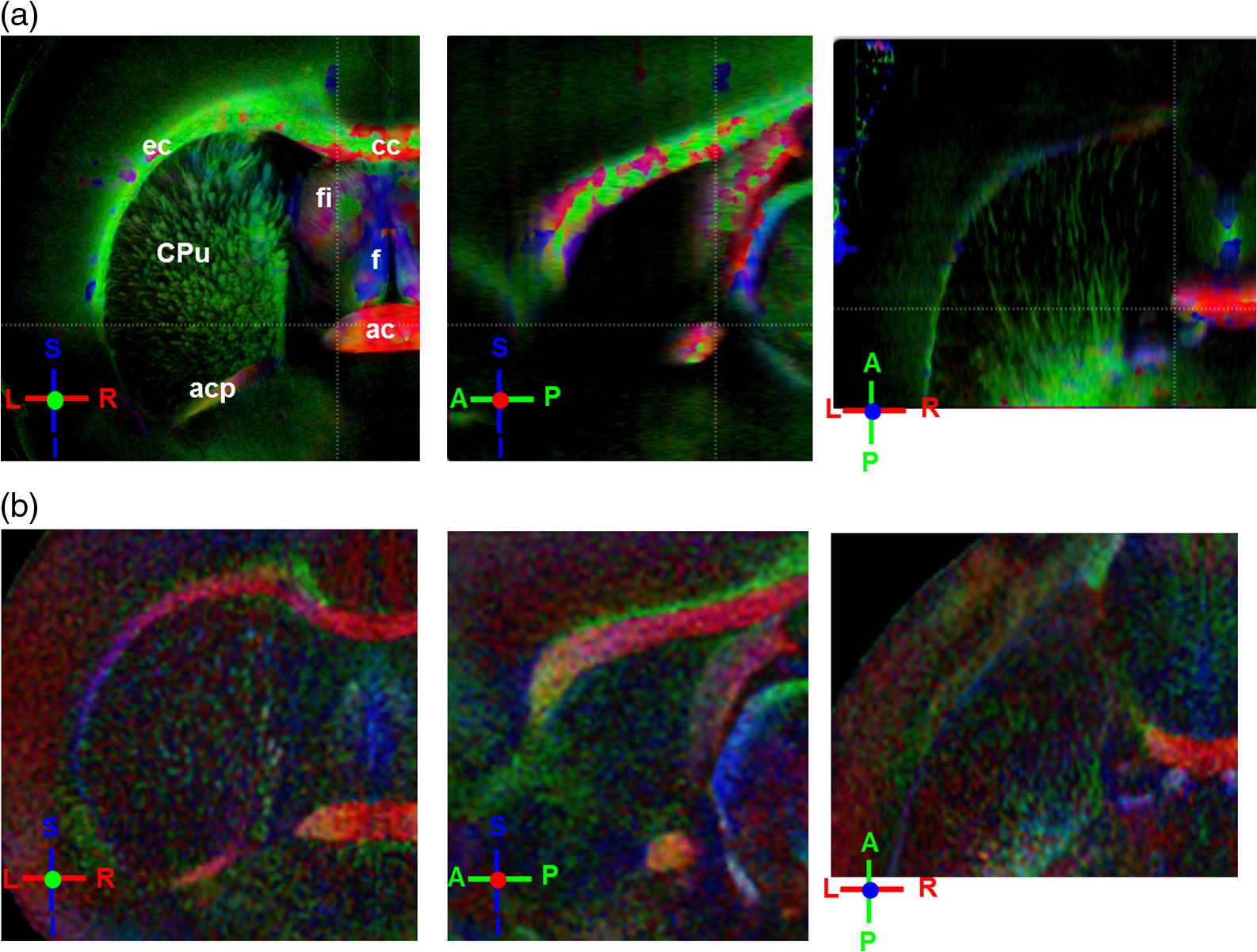 The 3-D dataset generated by stitching the volumetric optical sections of serial scans provides higher resolution for delineating the fiber map. ST analysis applied on this dataset provides a favorable solution for both large-scale orientation quantification and comprehensive connectivity investigations. To achieve more efficient computation, the dataset was downsampled to a voxel size of . Figure 6 shows a 3-D orientation map of the right hemisphere of a rat brain. The colors represent the orientations as follows: red: rostral-caudal, green: left-right, and blue: superior-inferior. The brightness is controlled by the pixel values of the cross-polarization images. Figure 6(a) illustrates the orthogonal views demonstrating fiber tracts with various directions and patterns. Directional changes of fiber tracts can be sensitively detected. On the coronal plane, the neural tracts through the putamen are aligned more horizontally in the lateral region (ROI 1) and vertically in the upper region (ROI 2). Similar color transitions are shown on the horizontal and sagittal planes. Moreover, results obtained from the 3-D ST analysis clarify the ambiguity of fiber alignments on 2-D ST images. For example, the orientation map on the horizontal plane shows that the fiber bundles in the ic run along the superior-inferior direction rather than the left-right direction which would be the apparent intuition from the 2-D plane. Fiber bundles aligned in the left-right direction are less visible, probably due to the fact that the optical systems barely detect the fibers along the illumination beam. This yields low backreflection and decreased signal intensity compared with the surrounding gray matter; therefore, some of the fiber bundles are not captured. Volume rendering of the 3-D orientation map is implemented in Vaa3D31 and shown in Fig. 6(b). Fig. 6The 3-D ST analysis on high-resolution reconstruction of rat brain. The dataset is generated by stitching the optical sections of the cross-polarization contrast. (a) Orthogonal views of the 3-D fiber orientations. ic: internal capsule. ROIs 1 and 2 indicate the fibers oriented along horizontal and vertical directions, respectively. The color sphere codes the orientations as red: anterior-posterior, green: left-right, and blue: superior-inferior. Directions are labeled on the orthogonal planes as well. Brightness is controlled by the dataset (cross-polarization). (b) Volume rending of the 3-D orientation map provides a perspective view.  The 3-D orientation obtained by ST analysis is not directly comparable with the optical measures as the optical axis orientation contrast in SOCS is restricted in 2-D. Therefore, we projected the 3-D computational orientation vectors onto the -plane and then generated en-face images to compare with the en-face optic axis orientation images. Pixel values on the en-face computational orientation image are determined by a histogram approach similar to that used for en-face optic axis orientation. Figure 7 shows the en-face images of a sagittal section. The computation (left) and the measurement (middle) are well correlated in most of the white matter, as shown by the absolute difference between the two images (right). Fiber orientations obtained by the two approaches closely match with the differences less than 10 deg in most regions where the image intensity is high and neural fibers are clearly traceable. These regions include the ic, the tracts in the putamen, the optic tract, the superior thalamic radiation, and the local fibers within the thamalus. More deviations are seen in the fiber bundles going through the plane. Fig. 7The 3-D orientation by ST analysis is (a) projected onto the -plane and (b) correlated with the en-face optic axis orientation. The color wheel indicates the orientations. The brightness is controlled by the en-face retardance values. The absolute difference of computed and measured orientations for pixels with retardance greater than 233 nm is plotted on the en-face retardance image (c). The color bar represents a narrow range (0 deg to 35 deg) for visualizing the mismatch.  3.4.TractographyTractography can be readily performed using the tools designed for diffusion MRI data. Figure 8 shows a representative tractography based on the ST analysis applied on the en-face retardance stack (). The tracts are color coded by their local orientations according to the directions shown in the cube (bottom-right corner). The original dataset is overlaid in grayscale for a better interpretation of the anatomy. Figure 8(a) illustrates the pathways beneath the cc. Only 14% of the tracts are shown due to the high density. Tracts in the mass white matter areas such as cc and ec are excluded, because the orientation estimation of the 3-D ST on these shell-like geometries does not align with the direction of its constituting fibers. To explore the fibers passing through a specific region, a sphere ROI indicated by a black arrow on Fig. 8(b) is placed at the conjunction of f and ac. The localization of the ROI is facilitated with the visualization of 3-D anatomical images of the en-face retardance stack. The tracts on Fig. 8(b) indicate that the fibers passing through this region primarily include f, fi, and ac. The ac is further branched in the anterior and posterior directions (aca and acp). Tracking of the ac is better visualized when the ROI is moved more laterally [Fig. 8(c)]. Fig. 8Tractography based on SOCS images. Tracts in color are computed from ST applied on the en-face stack of retardance. Colors in the cube represent the directions. Tracts are overlaid on the original data (grayscale). (a) Tracts excluding the cc and ec. Considering the high density, only 14% of the tracts are shown. (b) Fibers passing through a ROI at the junction between the ac and the f (gray sphere indicated by black arrow). (c) Fibers passing through another ROI (blue sphere) on the ac.  4.DiscussionAbnormalities of structure, orientation, and connectivity in the white matter have been linked to many brain diseases; however, comprehensive understanding of those factors with current imaging techniques is limited by spatial resolution or restricted coverage. In this paper, we demonstrated an ST approach to establish quantitative fiber orientation maps and the neuroanatomical connectivity in rat brain with SOCS imaging. This data-driven model offers a viable solution for comprehensive estimation of fiber orientations at microscopic resolution in complex brains. The eigenvectors of the ST sensitively capture the directionality of the anatomical features, and the computed orientation maps are well correlated with the measured in-plane optic axis orientation contrast of SOCS. Quantitative comparisons between the computed and measured orientations disclose an agreement with difference in the well delineated fiber tracts (Figs. 4 and 7). The 3-D fiber orientation maps obtained by ST provide details that have not been available with direct optical measures. Owing to the high resolution of SOCS images, fiber tracts of in diameter are visualized on the stitched optical sections. ST applied on this dataset produced the 3-D orientation of the fiber tracts (Fig. 6). Although the smooth kernel for ST computation inevitably undermines the image resolution, this effect can be minimized by controlling the kernel size on high-quality images. In the current analysis, the smoothing kernel size used for 3-D ST is , indicating that the orientations of the crossing fiber groups would not be distinguished within the neighborhood due to the averaging effect. However, the orientation estimation for the parallel fibers with smaller sizes (down to ) is still valid. Speckle noise on SOCS images is a dominant factor limiting the reliability of ST with smaller kernel size. Future improvements on the optical resolution and speckle-reduction techniques could enhance the results. In this study, we also applied the 3-D ST analysis on a stack of en-face retardance images. The dataset, although bearing a compromised resolution on the -axis, provides a global inspection of fiber organizations in the brain. The 3-D orientation map (Fig. 5) demonstrates the preferred orientations in the majority of the fiber tracts, where directionality of the structural features can be identified. Inconsistent estimations are seen in the cc and ec (blue embedded in red colors on Fig. 5), probably because the mass white matter regions form a shell-like geometry without showing the features of individual fiber bundles. As opposed to the cylindrical shape of individual fiber tracts which have a uniquely defined direction, the plenary structures lack a dominant direction. As a result, the ST estimation for the orientation merely shows a direction with the least local gradient, not necessarily parallel to the individual fiber direction. This problem might be solved by developing contrasts and enhancing the optical resolution for fiber identification. The comparison of the ST results and the optic axis orientation yields good agreement in well-defined fiber tracts. The discrepancies arise in the white matter regions where the fiber architectures are poorly depicted on the SOCS images. This could be caused by low retardance values, which typically imply the presence of fibers with low birefringence, running through the plane or crossing with each other. In these scenarios, the optic axis orientation measure bears more noise. The low contrast and the noisy features on the images affect the ST analysis making the fiber orientation estimation more prone to error. For instance, the small fiber tracts in the thalamus were barely visible due to low retardance; as a result, the ST estimation and the optic axis orientation measures may not be accurate and comparable with each other. Another example was found in the fiber bundles exiting the -plane with large angles, such as the cc in the sagittal sections, where the contrast between the white and gray matters was lost. This study concentrated on the myelinated fiber tracts due to the high birefringence of myelin sheath. SOCS imaging and ST analysis of unmyelinated fiber tracts that exhibit low birefringence require further investigation. The feature visibility with SOCS can be enhanced by the optical setup and the problems of the directional anisotropy of scattering and the dependence of measured retardance on the inclination angle of the neuronal fiber tracts could potentially be dealt with multidirectional illuminations. Angle-resolved imaging techniques have been suggested in OCT,35,36 and a polarization-sensitive OCT with variable-incidence angles has been reported to support 3-D orientation estimation.37 Another method is to improve the spatial resolution for feature identification.38,39 Incorporation of these techniques in SOCS imaging for drawing the full-angle wiring system in complex brains needs to be explored. The formation of the ST establishes a seamless connection to the tractography tools developed for diffusion MRI to investigate fiber tracking and structural connectivity. For proof of principle, we construct a tractography based on the en-face stack of retardance images. Excluding the cc and the ec, the tracts comply with the prior knowledge of anatomy (Fig. 8). We could also conduct the tractography on the high-resolution 3-D ST matrices, derived from the stitched optical sections in SOCS; however, the results need to be more delicately visualized and more carefully interpreted due to the high density of fiber pathways. Another concern is that the identification of the fiber tracts through the -plane is weaker than the fibers parallel to the -plane; therefore, the tract map could miss certain directions and induce a biased connectivity result. In summary, the combination of the ST analysis and the SOCS imaging provides a viable tool for brain-wide orientation mapping and connectome exploration at microscopic resolution. The 3-D orientation estimation from SOCS images enables a comprehensive cross-scale investigation with dMRI techniques.40 The method is easily generalized to other 3-D imaging techniques, including conventional OCT, serial microscopy,41,42 and light sheet microscopy,43 to support quantitative evaluation of fiber orientation where direct measure is not available. The analysis is also applicable to other tissues and molecular structures, in which anisotropic features are identified. The computational analysis provides an objective assessment of tissue microstructures, thus facilitating quantitative assessments of pathological studies. AcknowledgmentsThis work was supported by the Graduate School Doctoral Dissertation Fellowship at the University of Minnesota (to HW) and the grants from the U.S. National Institutes of Health: the National Institute of Biomedical Imaging and Bioengineering (R01 EB012538 and P41 EB015894) and the National Institute of Neurological Disorders and Stroke (P30 NS076408). We thank Minnesota Supercomputing Institute for the high-performance computing resources and the Duke Center for In Vivo Microscopy for providing the public online dataset of high-resolution diffusion tensor atlas of the rodent brain. ReferencesD. R. Fields,
“White matter in learning, cognition and psychiatric disorders,”
Trends Neurosci., 31 361
–370
(2008). http://dx.doi.org/10.1016/j.tins.2008.04.001 TNSCDR 0166-2236 Google Scholar
M. E. Thomason and P. M. Thompson,
“Diffusion imaging, white matter, and psychopathology,”
Annu. Rev. Clin. Psychol., 7 63
–85
(2011). http://dx.doi.org/10.1146/annurev-clinpsy-032210-104507 1548-5943 Google Scholar
P. J. Basser, J. Mattiello and L. D. Bihan,
“Estimation of the effective self-diffusion tensor from the NMR spin-echo,”
J. Magn. Reson. B, 103 247
–254
(1994). http://dx.doi.org/10.1006/jmrb.1994.1037 JMRBE5 1064-1866 Google Scholar
S. Mori and J. Zhang,
“Principles of diffusion tensor imaging and its applications to basic neuroscience research,”
Neuron, 51 527
–539
(2006). http://dx.doi.org/10.1016/j.neuron.2006.08.012 NERNET 0896-6273 Google Scholar
D. S. Tuch et al.,
“High angular resolution diffusion imaging reveals intravoxel white matter fiber heterogeneity,”
Magn. Reson. Med., 48
(4), 577
–582
(2002). http://dx.doi.org/10.1002/(ISSN)1522-2594 MRMEEN 0740-3194 Google Scholar
V. J. Wedeen et al.,
“Mapping complex tissue architecture with diffusion spectrum magnetic resonance imaging,”
Magn. Reson. Med., 54
(6), 1377
–1386
(2005). http://dx.doi.org/10.1002/(ISSN)1522-2594 MRMEEN 0740-3194 Google Scholar
P. C. Sundgren et al.,
“Diffusion tensor imaging of the brain: review of clinical applications,”
Neuroradiology, 46 339
–350
(2004). http://dx.doi.org/10.1007/s00234-003-1114-x 0028-3940 Google Scholar
S. Chanraud et al.,
“MR diffusion tensor imaging: a window into white matter integrity of the working brain,”
Neuropsychol. Rev., 20 209
–225
(2010). http://dx.doi.org/10.1007/s11065-010-9129-7 NERVEJ 1040-7308 Google Scholar
M. D. Budde et al.,
“The contribution of gliosis to diffusion tensor anisotropy and tractography following traumatic brain injury: validation in the rat using Fourier analysis of stained tissue sections,”
Brain, 134 2248
–2260
(2011). http://dx.doi.org/10.1093/brain/awr161 BRAIAK 0006-8950 Google Scholar
A. S. Choe et al.,
“Validation of diffusion tensor MRI in the central nervous system using light microscopy: quantitative comparison of fiber properties,”
NMR Biomed., 25 900
–908
(2012). http://dx.doi.org/10.1002/nbm.v25.7 NMRBEF 0952-3480 Google Scholar
Y. Wang et al.,
“Histology validation of mapping depth resolved cardiac fiber orientation in fresh mouse heart using optical polarization tractography,”
Biomed. Opt. Express, 5 2843
–2855
(2014). http://dx.doi.org/10.1364/BOE.5.002843 BOEICL 2156-7085 Google Scholar
D. Huang et al.,
“Optical coherence tomography,”
Science, 254 1178
–1181
(1991). http://dx.doi.org/10.1126/science.1957169 SCIEAS 0036-8075 Google Scholar
H. Wang et al.,
“Reconstructing micrometer-scale fiber pathways in the brain: multi-contrast optical coherence tomography based tractography,”
NeuroImage, 58 984
–992
(2011). http://dx.doi.org/10.1016/j.neuroimage.2011.07.005 NEIMEF 1053-8119 Google Scholar
J. B. Arous et al.,
“Single myelin fiber imaging in living rodents without labeling by deep optical coherence microsopy,”
J. Biomed. Opt., 16 116012
(2011). http://dx.doi.org/10.1117/1.3650770 JBOPFO 1083-3668 Google Scholar
C. Leahy, H. Radhakrishnan and V. J. Srinivasan,
“Volumetric imaging and quantification of cytoarchitecture and myeloarchitecture with intrinsic scattering contrast,”
Biomed. Opt. Express, 4 1978
–1990
(2013). http://dx.doi.org/10.1364/BOE.4.001978 BOEICL 2156-7085 Google Scholar
H. Wang, J. Zhu and T. Akkin,
“Serial optical coherence scanner for large-scale brain imaging at microscopic resolution,”
NeuroImage, 84 1007
–1017
(2014). http://dx.doi.org/10.1016/j.neuroimage.2013.09.063 NEIMEF 1053-8119 Google Scholar
J. Bigun and G. Granlund,
“Optimal orientation detection of linear symmetry,”
in Proc. IEEE First Int. Conf. on Computer Vision (ICCV),
433
–438
(1987). Google Scholar
T. Brox et al.,
“Adaptive structure tensors and their applications,”
Visualization and Processing of Tensor Fields, Springer Berlin, Heidelberg
(2006). Google Scholar
H. Haußecker and B. Jähne,
“A tensor approach for local structure analysis in multidimensional images,”
171
–1178 Erlangen, Germany
(1996). Google Scholar
R. Rezakhaniha et al.,
“Experimental investigation of collagen waviness and orientation in the arterial adventitia using confocal laser scanning microscopy,”
Biomech. Model. Mechanobiol., 11 461
–473
(2012). http://dx.doi.org/10.1007/s10237-011-0325-z BMMICD 1617-7959 Google Scholar
M. Krause et al.,
“Determination of the fibre orientation in composites using the structure tensor and local x-ray transform,”
J. Mater. Sci., 45 888
–896
(2010). http://dx.doi.org/10.1007/s10853-009-4016-4 JMTSAS 0022-2461 Google Scholar
O. Schmitt et al.,
“Analysis of nerve fibers and their distribution in histologic sections of the human brain,”
Microsc. Res. Tech., 63 220
–243
(2004). http://dx.doi.org/10.1002/(ISSN)1097-0029 MRTEEO 1059-910X Google Scholar
O. Schmitt and H. Birkholz,
“Improvement in cytoarchitectonic mapping by combining electrodynamic modeling with local orientation in high-resolution images of the cerebral cortex,”
Microsc. Res. Tech., 74 225
–243
(2011). http://dx.doi.org/10.1002/jemt.v74.3 MRTEEO 1059-910X Google Scholar
M. D. Budde and J. A. Frank,
“Examining brain microstructure using structure tensor analysis of histological sections,”
NeuroImage, 63 1
–10
(2012). http://dx.doi.org/10.1016/j.neuroimage.2012.06.042 NEIMEF 1053-8119 Google Scholar
H. Wang, M. K. Al-Qaisi and T. Akkin,
“Polarization-maintaining fiber based polarization-sensitive optical coherence tomography in spectral domain,”
Opt. Lett., 35 154
–156
(2010). http://dx.doi.org/10.1364/OL.35.000154 OPLEDP 0146-9592 Google Scholar
J. Bigun, T. Bigun and K. Nilsson,
“Recognition by symmetry derivatives and the generalized structure tensor,”
IEEE Trans. Pattern Anal. Mach. Intell., 26
(12), 1590
–1605
(2004). http://dx.doi.org/10.1109/TPAMI.2004.126 ITPIDJ 0162-8828 Google Scholar
D. J. Kroon and C. H. Slump,
“Coherence filtering to enhance the mandibular canal in cone-beam CT data,”
in Proc. 4th Annual Symp. of the IEEE-EMBS Benelux Chapter,
41
–44
(2009). Google Scholar
R. Wang et al.,
“Diffusion Toolkit: a software package for diffusion imaging data processing and tractography,”
in Proc. Intl. Soc. Mag. Reson. Med.,
3720
(2007). Google Scholar
P. J. Basser et al.,
“In vitro fiber tractography using DT-MRI data,”
Magn. Reson. Med., 44 625
–632
(2000). http://dx.doi.org/10.1002/(ISSN)1522-2594 MRMEEN 0740-3194 Google Scholar
S. Mori et al.,
“Three-dimensional tracking of axonal projections in the brain by magnetic resonance imaging,”
Ann. Neurol., 45 265
–269
(1999). http://dx.doi.org/10.1002/(ISSN)1531-8249 ANNED3 0364-5134 Google Scholar
D. Weinstein, G. Kindlmann and E. C. Lundberg,
“Tensorlines: advection diffusion based propagation through diffusion tensor fields,”
in In Proc. of the Conf. on Visualization (VIS’99): celebrating ten years,
249
–253
(1999). Google Scholar
G. A. Johnson et al.,
“A multidimensional MR histology atlas of the Wistar rat brain,”
NeuroImage, 62 1848
–1856
(2012). http://dx.doi.org/10.1016/j.neuroimage.2012.05.041 NEIMEF 1053-8119 Google Scholar
J. Veraart et al.,
“Population-averaged diffusion tensor imaging atlas of the Sprague Dawley rat brain,”
NeuroImage, 58 975
–983
(2011). http://dx.doi.org/10.1016/j.neuroimage.2011.06.063 NEIMEF 1053-8119 Google Scholar
H. Peng et al.,
“V3D enables real-time 3D visualization and quantitative analysis of large-scale biological image data sets,”
Nat. Biotechnol., 28 348
–353
(2010). http://dx.doi.org/10.1038/nbt.1612 NABIF9 1087-0156 Google Scholar
J. W. Pyhtila, R. N. Graf and A. Wax,
“Determining nuclear morphology using an improved angle-resolved low coherence interferometry system,”
Opt. Express, 11 3473
–3484
(2003). http://dx.doi.org/10.1364/OE.11.003473 OPEXFF 1094-4087 Google Scholar
M. G. Giacomelli and A. Wax,
“Imaging beyond the ballistic limit in coherence imaging using multiply scattered light,”
Opt. Express, 19 1285
–1287
(2011). http://dx.doi.org/10.1364/OE.19.004268 OPEXFF 1094-4087 Google Scholar
Z. Lu, D. K. Kasaragod and S. J. Matcher,
“Optic axis determination by fibre-based polarization-sensitive swept-source optical coherence tomography,”
Phys. Med. Biol., 56 1105
–1122
(2011). http://dx.doi.org/10.1088/0031-9155/56/4/014 PHMBA7 0031-9155 Google Scholar
V. J. Srinivasan et al.,
“Optical coherence microscopy for deep tissue imaging of the cerebral cortex with intrinsic contrast,”
Opt. Express, 20 2220
–2239
(2012). http://dx.doi.org/10.1364/OE.20.002220 OPEXFF 1094-4087 Google Scholar
C. Magnain et al.,
“Blockface histology with optical coherence tomography: a comparison with Nissl staining,”
NeuroImage, 84 524
–533
(2014). http://dx.doi.org/10.1016/j.neuroimage.2013.08.072 NEIMEF 1053-8119 Google Scholar
H. Wang et al.,
“Cross-validation of serial optical coherence scanning and diffusion tensor imaging: a study on neural fiber maps in human medulla oblongata,”
NeuroImage, 100 395
–404
(2014). http://dx.doi.org/10.1016/j.neuroimage.2014.06.032 NEIMEF 1053-8119 Google Scholar
G. B. Sands et al.,
“Automated imaging of extended tissue volumes using confocal microscopy,”
Microsc. Res. Tech., 67 227
–239
(2005). http://dx.doi.org/10.1002/(ISSN)1097-0029 MRTEEO 1059-910X Google Scholar
T. Ragan et al.,
“Serial two-photon tomography for automated ex vivo mouse brain imaging,”
Nat. Methods, 9 255
–258
(2012). http://dx.doi.org/10.1038/nmeth.1854 1548-7091 Google Scholar
P. J. Keller et al.,
“Reconstruction of zebrafish early embryonic development by scanned light sheet microscopy,”
Science, 322 1065
–1069
(2008). http://dx.doi.org/10.1126/science.1162493 SCIEAS 0036-8075 Google Scholar
BiographyHui Wang received her BS and MS degrees in electrical engineering from the Huazhong University of Science and Technology, China, in 2006 and 2008, respectively, and her PhD degree in biomedical engineering from the University of Minnesota in 2014. Her research interests include optical coherence tomography, optical imaging on biomedical applications, neuroimaging, and signal processing. Christophe Lenglet is a McKnight Land-Grant Assistant Professor in the Department of Radiology at the University of Minnesota. He is a faculty member of the Center for Magnetic Resonance Research and a scholar of the Institute for Translational Neuroscience. His lab develops computational tools to harness the power of high-field magnetic resonance imaging for neuroscience and clinical applications. His research aims at better understanding the structural and functional alterations of brain connections in neurodegenerative disorders. Taner Akkin received his BSc (1995) and MSc (1997) degrees in electrical and electronics engineering from Çukurova University, Turkey, and his PhD degree (2003) from the University of Texas at Austin. After postdoctoral studies at Harvard Medical School/Wellman Center for Photomedicine, Massachusetts General Hospital, he joined the Department of Biomedical Engineering at the University of Minnesota (2005), where he is an associate professor. He develops optical imaging systems to study neural structure and function. |


