2.1.

Caenorhabditis Elegans Muscles

Although many studies have explored the basic functioning of muscles and their components, important aspects of sarcomere assembly and the contractile process are still not fully understood. C. elegans represents an attractive model system for microscopy studies³³ on muscular function, because it presents large-sized sarcomeres.³⁴ It also possesses the two types of muscle: striated and nonstriated. The obliquely striated body-wall muscles of this nematode consist of multiple sarcomeres, similar to the skeletal muscles in vertebrates.³⁵ The nonstriated, single-sarcomere muscle cells are analogous to cardiac muscle cells in mammals and include the pharyngeal group.³⁵

The sarcomere consists of three differentiated regions. The isotropic (I) half-bands correspond to thin filaments made of actin; an anisotropic (A) band includes an overlapping region of thick filaments with thin filaments; the M-line, in the middle of the sarcomere, contains only thick filaments. The elements responsible for the SHG signal inside the sarcomere are the thick filaments.¹⁷ These are rigid structures based on a tubule-like core that constitutes the backbone of the filament.^{36, 37, 38} The internal density of the filament core appears hollow at the poles (similar to collagen type I fibrils),³⁹ and they are made up of double-helix chiral myosin rods and heads. An interaction between the myosin heads and actin filaments produces muscle contraction and tension.

It has been reported that the SHG source in muscle lies in the rod domain of myosin’s double helix, and that the myosin heads do not contribute to the signal.¹⁷ Furthermore, electron microscopy has shown that the spatial arrangement of thick filaments in the body walls, in the transverse direction, follows a hexagonal architecture.³³ Based on this evidence, our model attributes hexagonal symmetry to the nonlinear susceptibility tensor in the sample.

2.2.

Worm Mounts

The strain juIs76 [unc-25::gfp] II was cultured and grown in large quantities using methods reported by S. Brenner.⁴⁰ The use of this specific strain relates to other research interests, but it is suitable for SHG muscular imaging because it only expresses green fluorescent protein (GFP) in a specific set of neurons. A number of healthy adult hermaphrodites were mounted on a 2% agar pad with $0.8\mu \mathrm{l}$ of $25\text{-}\mathrm{mM}$ sodium azide (NaN3) between two $40\text{-}\mu \mathrm{m}$ glass slides. The choice of this specific anesthesia allowed us to fully immobilize the worms, and therefore reduce motion artifacts. The mounts were sealed with melted paraffin for stabilization and were only used for a period of less than half an hour to guarantee the physical condition of the worms. The laboratory temperature was $21°\mathrm{C}$ .

2.3.

Experimental Setup

The experimental setup was based on an adapted inverted microscope (Nikon TE2000-U) with the $y\text{-}z$ scanning unit composed of a pair of galvanometric (galvo) mirrors. A labVIEW interface program was written to control the raster scanning of the galvanometric mirrors and the data acquisition (DAQ) card. Typical frame acquisition times for a single $500\times 500\text{pixel}$ image were about $1\text{to}2\mathrm{s}$ . Two $60\times$ oil-immersion objectives [numerical aperture $\left(\mathrm{NA}\right)=1.4$ , Nikon Plain Apo-Achromatic] were used throughout the experiments for excitation and collection of the nonlinear signals.

For the excitation source, we used a Kerr lens mode-locked Ti:sapphire laser (MIRA 900f), which delivers pulses of $160\mathrm{fs}$ and operates at a central wavelength of $840\mathrm{nm}$ with a repetition rate of $76\mathrm{MHz}$ . The average power reaching the sample plane was controlled (using neutral density filters) to be in the range of $20\text{to}30\mathrm{mW}$ . With this regime, no observable damage occurred for long imaging periods of time. We placed a linear polarizer after the galvo mirrors to eliminate any ellipticity or depolarization introduced from the setup. This was followed by a half-wave plate that was rotated in steps to change the polarization at the sample plane. For the analysis, we defined the lab $z$ axis in the horizontal direction in our images. This corresponded to the angle origin $(\alpha =0)$ of the incoming linear polarization. Subsequent linear polarizations were used by rotating them clockwise in steps of $20\mathrm{deg}$ . Finally, we assessed the effect of several optical components in our microscope placed before the sample plane (galvo mirrors, lenses, half-wave plate, dichroic mirror, and objective) on the depolarization of the fundamental beam. This was done by measuring the power of the fundamental beam as a function of the rotation angle of an analyzer placed at the microscope sample plane and before the power meter. We found that the fundamental input average power showed an extinction coefficient ratio of 25:1 under rotation of the input polarization.

Since the great majority of the SHG signal generated from muscular tissues is forward propagated, a proper mount and detection unit was implemented in this direction. This unit contained the collecting high numerical aperture $(\mathrm{NA}=1.4)$ objective, a BG39 filter, a $10\text{-}\mathrm{nm}$ FWHM band-pass filter centered at $420\mathrm{nm}$ and a photomultiplier tube (PMT). The objective lens was mounted on a micrometric 3-D translational stage with tilt correction, and the whole unit was enclosed to minimize stray or spurious light into the PMT.

2.4.

PSHG Biophysical Model

Our generalized biophysical model is based on those proposed previously.^{14, 15, 16, 17, 18} For clarity, we describe it here while introducing the generalization, which allows the acquisition of any arbitrary orientation $\varphi$ of the thick filaments.

Our model first considers that the SHG active volume in our experiment $(\sim 0.1\mu {\mathrm{m}}^2\times 0.8\mu \mathrm{m})$ is smaller than the size of a sarcomere, but it includes several thick filaments (considered the source of SHG signal in muscle¹⁷) that are hexagonally arranged.³³ Therefore, a spatial symmetry corresponding to hexagonal crystal system is assumed. Second, we further consider that the thick filaments are at an arbitrary angle orientation and parallel to the sample plane of the microscope (see Fig. 1 ).

Fig. 1

Schematic representation of coordinate system inside the focusing volume. The beam propagates along the $x$ direction, and the main symmetry axis is in an angle $\varphi$ with the $z$ axis. $\alpha$ is the angle of the incoming linear polarization with the $z$ axis. Cylinders represent thick filaments, and the shadowed region corresponds to the SHG active volume. Figure is not on a predefined scale.

To be formally correct, we assume that the local hexagonal arrangement of thick filaments was transduced in a $C_6$ crystal class whose susceptibility tensor in its contracted notation is given by⁴¹

We further consider a linear polarization of the incident electric field in which no axial component $E_{x^{\prime }}^{\omega }$ is introduced by our high-NA $(\mathrm{NA}=1.4)$ objective. In our experiment the polarization is rotated clockwise with an angle $\alpha$ measured with respect to the $z$ axis (lab macroscopic frame). The amplitude of the electric field at the focal position, expressed in the thick filaments coordinate frame, is given by

2.5.

Single-Axis Molecule Approach

By expanding the model to the microscopic (molecular) frame and by considering a coherent summation of the molecular hyperpolarizability tensor ${\beta }_{i^{″}{j}^{″}{k}^{″}}$ , the different elements in the macroscopic nonlinear susceptibility tensor can be obtained. In addition, it is generally assumed that the single-axis molecules posses a unique nonvanishing element ${\beta }_{z^{″}{z}^{″}{z}^{″}}=\beta$ .^{17, 18, 42} Then the components of the susceptibility tensors are obtained:

By considering a molecular random distribution in the azimuth angle ( $\phi )$ , then $D(\theta ,\phi )=D\left(\theta \right)$ , and Eq. 11 reduces to ${\chi }_{31}^{\left(2\right)}={\chi }_{15}^{\left(2\right)}=\beta N⟨\cos \theta {\sin }^2\theta ⟩∕2$ . Equivalently, Eq. 12 would result in ${\chi }_{14}^{\left(2\right)}=0$ . However, this aspect cannot be corroborated since our model is not able to retrieve information on this tensor element.

Finally, assuming a square distribution for $D\left(\theta \right)$ , the mean effective molecule or harmonophore orientation can be estimated as^{18, 42}

2.6.

Fitting Method

In order to make apparent the fitting process, Eq. 8 is rewritten as

The difference between Eqs. 8, 14 is in the extra term $\Delta$ . This parameter has been added to include both experimental errors and any deviation from the theoretical model, so it is not to be considered a simple background contribution. This is because the minimum value in Eq. 14, without considering any background, can be larger than zero depending on the actual values of $a$ and $b$ . This makes it difficult to a priori quantify the contribution of $\Delta$ to the detected signal. In addition, $\Delta$ can slightly change from pixel to pixel. Therefore, it has been included as a free parameter in the fitting algorithm.

Our fitting algorithm produces an intrinsic indetermination. This occurs because when $a={\chi }_{31}^{\left(2\right)}∕{\chi }_{15}^{\left(2\right)}$ and $b={\chi }_{33}^{\left(2\right)}∕{\chi }_{15}^{\left(2\right)}$ , it gives the same result at $\varphi$ as $b={\chi }_{31}^{\left(2\right)}∕{\chi }_{15}^{\left(2\right)}$ and $a={\chi }_{33}^{\left(2\right)}∕{\chi }_{15}^{\left(2\right)}$ at $\varphi +\pi ∕2$ . To solve this, we imposed the condition that the larger of the two coefficients $a$ or $b$ given by the fitting algorithm must correspond to ${\chi }_{31}^{\left(2\right)}∕{\chi }_{15}^{\left(2\right)}$ , and the remaining coefficient and angle must be chosen accordingly. This assumption is correct only in the case of muscle¹⁸ and therefore must be revised for other SHG active structures. In addition, since all the terms in Eq. 8 are positive, the algorithm is forced to retrieve positive real values for all the parameters in Eq. 14. Thus, spurious solutions, usually with negative values for either $a$ or $b$ and $\Delta$ , are avoided.

Having implemented all these observations, we applied our fitting algorithm to each pixel of a selected region of interest (ROI). This was done after applying a low-pass filter (equivalent to averaging the four surrounding neighboring pixels) to remove any possible small-moving artifacts. The average intensity among five different images of the same plane and polarization was used to obtain an accurate analysis. Under these conditions, over 1000 iterations per pixel were used to adjust the experimental data to the model. The free image processing software Image J (National Institutes of Health) was used for image treatment.

3.1.

Considerations of the Theoretical Model

Three important considerations have not yet been considered by our model: (1) the SHG signal reaching the collecting objective with off-axis $\widehat{k}$ vectors (within the NA); (2) the change of the polarization state (existence of axial components) due to the high-NA objective, and (3) the effect of thick filaments tilted off-plane. The consideration of off-axis $\widehat{k}$ vectors and a close equation for the intensity,⁴³ are making the analysis numerically complex The two remaining aspects, axial field components and off-plane filaments, could be included in the model by adding an extra $\psi$ angle to complete the Euler set of angles and by using analyzers in detection to determine this angle.⁴² All this would also incorporate the ${\chi }_{14}^{\left(2\right)}$ tensor element in our model, whose inclusion would add complexity to the model by introducing extra ambiguities into the equation.

In view of the above discussion, we decided to keep our simpler approach and instead to analyze how these three factors could affect our results. In all three cases, the main effect is expected to be an extra contribution of the nonlinear polarization component $P_{x^{\prime }}^{2\omega }$ to the detected SHG signal (although $P_{y^{\prime }}^{2\omega }$ and $P_{z^{\prime }}^{2\omega }$ can also change). In principle, this SHG signal due to $P_{x^{\prime }}^{2\omega }$ would drop very fast (nonlinearly) and could be a priori disregarded. However, our fitting algorithm has the potential to consider its contribution and to minimize its impact on the retrieved results thanks to the inclusion of the $\Delta$ parameter.

The experimental background (electronic noise, nonfiltered fundamental signal, or external light) can be estimated by measuring the intensity in regions without any SHG signal. This corresponds to $\sim 1\%$ of the detected signal. However, the value of the $\Delta$ parameter is larger and can change from pixel to pixel. Typically, in an image, $\Delta$ is around 20% of the detected signal with a change of 2 to 3% from pixel to pixel. Its nature can be associated with the causes mentioned above, as well as the existence of other factors such as two-photon fluorescence. A certain dependence of $\Delta$ with the incoming polarization is expected. However, when determining $\Delta$ , the fitting algorithm does not take into account this dependence, so it gives an average value. As a consequence, the fitting algorithm removes part of the unwanted contributions included in $\Delta$ . This is shown in Figs. 3b, 4b, 5b, where the quality of fitting for most of the pixels was above 85%; when $\Delta$ was not included, the quality of fitting was always below 70%.

Fig. 3

Algorithm fitting results: (a) Average intensity of all the SHG images shown in Fig. 2. The red square shows the ROI where the fitting algorithm was applied. Scale bar corresponds to $10\mu \mathrm{m}$ . (b) Quality of fitting $\left(r^2\right)$ . (c) and (d) Obtained ratios between the elements of the ${\chi }^{\left(2\right)}$ tensor. (e) Orientation of thick filaments $\left(\varphi \right)$ . (f) Effective orientation of harmonophores $\left({\theta }_e\right)$ , both in degrees. For clarity, the values with a quality of fitting $\left(r^2\right)$ inferior to 95% were rejected from the figures. (Color online only.)

Fig. 4

Results of fitting the algorithm to body walls oriented at an arbitrary inclination angle. (a) Average intensity of nine different PSHG images (each step in the incoming linear polarization is $20\mathrm{deg}$ ). Scale bar is $10\mu \mathrm{m}$ . (b) Coefficient of determination $\left(r^2\right)$ . (c) $a={\chi }_{31}^{\left(2\right)}∕{\chi }_{15}^{\left(2\right)}$ and (d) $b={\chi }_{33}^{\left(2\right)}∕{\chi }_{15}^{\left(2\right)}$ are obtained ratios between the elements of the ${\chi }^{\left(2\right)}$ tensor. (e) Orientation of thick filaments $\left(\varphi \right)$ . Arrow indicates real inclination at $58.47\mathrm{deg}$ . (f) Effective orientation of harmonophores $\left({\theta }_e\right)$ in degrees.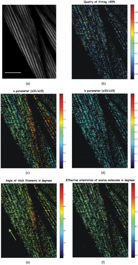

Fig. 5

(a) Average intensity of nine different PSHG images (each step in the incoming linear polarization is $20\mathrm{deg}$ ) of the C. elegans terminal (posterior) lobe of the pharynx. Scale bar is $10\mu \mathrm{m}$ . This image corresponds to a longitudinal section of the lobe where the grinder is located. The posterior of the worm is upper left and the anterior is lower right. (b) Coefficient of determination $\left(r^2\right)$ . (c) $a={\chi }_{31}^{\left(2\right)}∕{\chi }_{15}^{\left(2\right)}$ and (d) $b={\chi }_{33}^{\left(2\right)}∕{\chi }_{15}^{\left(2\right)}$ are obtained ratios between the elements of the ${\chi }^{\left(2\right)}$ tensor. (e) Orientation of thick filaments $\left(\varphi \right)$ . Arrows indicate real inclination and their colors represent the intervals of the degree color map on the top. The white arrow indicates the position of the grinder system. (f) Harmonophore orientation $\left({\theta }_e\right)$ in degrees.

A final remark on the method concerns Kleinman’s symmetry conditions. In our experiments, these conditions imply that ${\chi }_{14}^{\left(2\right)}=0$ and ${\chi }_{31}^{\left(2\right)}={\chi }_{15}^{\left(2\right)}$ . The determination of the ${\chi }_{31}^{\left(2\right)}∕{\chi }_{15}^{\left(2\right)}$ ratio can give a measure of the validity of those conditions. In our case, Figs. 3c, 4c, 5c show that a large number of pixels returned an $a$ -parameter value that was different from unity. This is an unexpected result if Kleinman’s conditions hold. To further check this fact, the fitting algorithm was run by assuming Kleinman’s symmetry conditions, i.e., ${\chi }_{31}^{\left(2\right)}∕{\chi }_{15}^{\left(2\right)}=1$ . The results showed a much lower quality of fitting (below 60%). In addition, the SHG signal at $\lambda =420\mathrm{nm}$ was very close to the resonant wavelength of the muscle at $\lambda \sim 430\mathrm{nm}$ .⁴⁴ Thus, care must be taken before assuming Kleinman’s symmetry conditions in experiments of this type.

3.2.

Caenorhabditis Elegans Body Walls

In vivo, PSHG imaging of C. elegans body wall muscles for nine different incoming polarizations are shown in Fig. 2 . Each image presented in this figure was composed by the mean intensity of five different images of the same polarization. As expected, there was clear variation of the intensity among the different SHG images. In this set of experiments, we found that the minimum PSHG intensity was observed when the incoming polarization was almost parallel with the thick filament orientation. Our results showed that the distinctive intensity PSHG fingerprint curve characteristic of muscle (result not shown) were in agreement to previous results in which myofibrils were oriented parallel to one axis of the coordinate system.^{14, 15, 16, 17, 18, 19, 21}

Fig. 2

Polarization-dependent SHG images of C. elegans ventral quadrants of body wall muscles. Incoming linear polarization is indicated by arrows and is rotating in steps of $20\mathrm{deg}$ . Scale bar shows 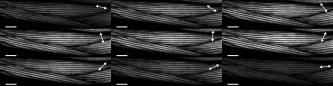$10\mu \mathrm{m}$ .

In this section, we analyze the images using pixel resolution. This is in contrast to previous PSHG studies on muscle where the results were obtained by averaging the intensity from large ROIs.^{14, 15, 16, 17, 18, 19, 21} Averaging over bigger regions would give smoother changes among any retrieved values.

We start by using the results in Fig. 2 to run our pixel resolution fitting algorithm to the selected ROI (where the thick filaments are mainly parallel to the $z$ axis), shown in Fig. 3a . Figure 3b shows the pixels that were fitted with a coefficient of determination of $r^2⩾95\%$ inside the selected ROI. Figures 3c, 3d, 3e, 3f show the $a$ and $b$ parameters, the angle of thick filaments, and the effective orientation of harmonophores, respectively. In these figures, large homogenous regions are shown (indicated with the same color) for the different parameters of the model. As commented previously, Fig. 3c exhibits some deviation from the situation ${\chi }_{31}^{\left(2\right)}∕{\chi }_{15}^{\left(2\right)}=1$ necessary for Kleinman’s symmetry to hold, with the majority of the pixels being around 1.4. For the structurally sensitive coefficient ${\chi }_{33}^{\left(2\right)}∕{\chi }_{15}^{\left(2\right)}$ , the ratio obtained for the majority of the pixels was at 0.45 [Fig. 3d]. These values are in agreement with those previously reported for myofibrils.^{14, 15, 16, 17, 18, 19} Figure 3e clearly shows that the retrieved angle $\varphi$ of thick filaments coincides well with the geometrical inclination observed in the ROI of Fig. 3a (angles between 0 and $5\mathrm{deg}$ ). Figure 3f shows the effective orientation angle of the harmonophores calculated using Eq. 13. The maximum number of pixels presented an angle in the region of $64.1\mathrm{deg}$ . These results will be discussed further later.

In the next step, the C. elegans body wall muscles were examined at an arbitrary inclination with respect to the $z$ axis [see Fig. 4a ]. In this way, it was possible to test if the generalization of the model including the angle $\varphi$ was valid. To do that, we followed the same procedure as before. It was found that the PSHG fingerprint curve^{14, 15, 16, 17, 18, 19, 21} was shifted according to the angle $\varphi$ . The results of the fitting for $r^2>85\%$ are depicted in Figs. 4b, 4c, 4d, 4e, 4f. The values of the different parameters are at the same intervals as those acquired before (body walls parallel to the $z$ axis). The maximum number of pixels for the $a$ , $b$ , and ${\theta }_e$ parameters was in the regions of 1.03, 0.38, and $65.5\mathrm{deg}$ , respectively. In the case of the angle $\varphi$ [Fig. 4e], the majority of the pixels showed an inclination for the thick filaments of $58.47\mathrm{deg}$ —very close to the real geometrical inclination in the SHG image. This clearly indicates that the method can correctly assess the orientation of thick filaments, and therefore, the sample does not need special alignment before starting the measurements. This advantage is crucial, especially when examining complex architectures, since it allows the simultaneous pixel resolution mapping of different orientations in the same image.

3.3.

Complex Thick Filament Architectures: The Terminal Lobe of the Caenorhabditis Elegans Pharynx

Although the orientation of the thick filaments in body walls could be easily predicted, in more complex structures such as the pharynx, the analysis should provide information not apparent from conventional SHG intensity imaging. Thus, our next objective was to analyze complex muscular structures that possess different orientations of the thick filaments in the same image.

The pharynx of C. elegans was used to approach this issue. The pharynx is a single, unified, epithelial bilobed organ composed of 20 cells, and it can be divided into eight distinct muscle groups, each containing one to three cells. Within the pharynx we selected a $y\text{-}z$ plane of a region in the most posterior lobe (the terminal bulb). This specific region of the pharynx was selected because it includes cells from three different muscle groups (pm5, pm6, and pm7) with different filament orientations. Moreover, the posterior lobe of the C. elegans pharynx has a highly complex organized structure where the muscular cells are organized on a threefold radial symmetry, with marginal cells in between, that rotate under contraction and allow for both a longitudinal and radial component to the motion of the grinder teeth (housed in the posterior lobe) during food intake.³³

To test the ability of our model to map the different orientations of the thick filaments in the same image, we performed the PSHG image analysis to the pharynx (see Fig. 5 ). The results of the fitting for the several structurally sensitive parameters of the model can be seen in Figs. 5c, 5d, 5e, 5f. In these figures, only values of $r^2>90\%$ are presented [Fig. 5b]. The maximum number of pixels for the $a$ , $b$ , and ${\theta }_e$ parameters was found at the values of 0.94, 0.52, and $63.02\mathrm{deg}$ , respectively. Figure 5e shows the obtained values for the angle $\varphi$ , which clearly demonstrates the radial distribution of thick filaments present in the most peripheral regions of both pm6 and pm7. Also in this figure, the pixel-by-pixel fitting of the algorithm resulted in a number of homogenous regions (shown with the same color or totally black). These regions are indicative of different angle orientations (different colors) or different structural characteristics (black) that did not fit to the algorithm. In all these cases, the different homogeneous regions can be distinguished from nearby regions. In the case of differently color regions, the obtained angle orientation hints at the local contraction direction of the sarcomere. Moreover, the fact that it is possible to choose coefficients of determination larger than a predefined value offers a new way of gaining contrast, because it filters PSHG pixels that do not fit to the model. Here, this fast was used to segment among different architectures. For example, using $r^2>90\%$ allowed us to uncover the several parts of muscular cells that control this nematode’s grinder in the pumping system (white arrow in Fig. 5). This information could not be reached with $r^2<90\%$ (data not shown) or by our conventional intensity SHG images [see Fig. 5a]. Also, the above result would not have been achieved without the generalization of the model (which allows mapping of different orientations of thick filaments in the same image) and without applying it at the pixel-by-pixel level.

3.4.

Effective Orientation of SHG Active Molecules

Since the effective orientation of the harmonophores [see Eq. 13 and Figs. 3f, 4f, 5f] is measured with respect to the thick filament, such angles have been associated with the helical pitch of myosin.^{17, 18} Such an association was made only after analyzing images of homogeneous striated fibrilar muscle samples in large ROIs and by assuming a square distribution of molecular orientations. In contrast, our pixel-resolution procedure allows for nonhomogeneous regions to be analyzed as the different structural parameters are obtained in a pixel-by-pixel basis. Therefore, the statistical molecular distribution $D\left(\theta \right)$ in a single pixel is expected to be narrower. As a consequence, it is more appropriate to consider the local distribution in Eqs. 10, 11, 12 as a Dirac delta. As previously mentioned, the effective angle ${\theta }_e$ given by Eq. 13 is then expected to be closer to the actual harmonophore orientation in the pixel. This further allows us to experimentally estimate the actual distribution of effective molecular orientations in the whole image. Thus, we calculated the frequency distribution of the angles given by Eq. 13 for our data [Figs. 3f, 4f, 5f]. These results, together with the frequency distribution corresponding to parameters $a={\chi }_{31}^{\left(2\right)}∕{\chi }_{15}^{\left(2\right)}$ and $b={\chi }_{33}^{\left(2\right)}∕{\chi }_{15}^{\left(2\right)}$ , are shown in Fig. 6 .

Fig. 6

Frequency distribution for the retrieved parameters: (a) $a={\chi }_{31}^{\left(2\right)}∕{\chi }_{15}^{\left(2\right)}$ , (b) $b={\chi }_{33}^{\left(2\right)}∕{\chi }_{15}^{\left(2\right)}$ , and (c) harmonophores orientation $\left({\theta }_e\right)$ corresponding to Figs. 3, 4, 5.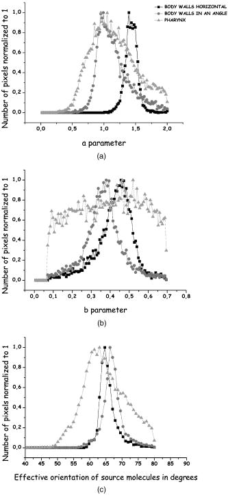

The frequency distribution for the ratio ${\chi }_{31}^{\left(2\right)}∕{\chi }_{15}^{\left(2\right)}$ shown in Fig. 6a exhibits a “well-behaved” bell-shaped distribution in all cases. The FWHM is similar in the horizontal body walls and the body walls in an angle, but broader for the pharynx (even if a smaller ROI is considered). This broadening also occurs in the frequency distribution of the ratio ${\chi }_{33}^{\left(2\right)}∕{\chi }_{15}^{\left(2\right)}$ [Fig. 6b] and as expected, in the frequency distribution of the effective orientation of harmonophores [Fig. 6c]. In this last case, the FWHM of such distribution, $\delta {\theta }_e$ , is indicative of the degree of disorganization of the SHG source molecules. However, $\delta {\theta }_e$ for the horizontal body walls and for those in an angle were found to be similar, $\sim 5\mathrm{deg}$ , while for the pharynx $\delta {\theta }_e$ was $\sim 15\mathrm{deg}$ . These $\delta {\theta }_e$ were narrow enough to allow the accurate determination of the mean ${\theta }_e$ found in other works.⁴⁵ The nature of the broader $\delta {\theta }_e$ in the pharynx might be attributed not only to the fact that thick filaments are not well organized, but also because some of these thick filaments may also tilted off of the sample plane.

The single-axis-molecules approach also imposes a ratio of ${\chi }_{31}^{\left(2\right)}∕{\chi }_{15}^{\left(2\right)}=1$ . As shown in Fig. 6a, the body walls in an angle [Fig. 4c] and the pharynx lobe [Fig. 5c] are centered at ${\chi }_{31}^{\left(2\right)}∕{\chi }_{15}^{\left(2\right)}=1$ . This is not the case for the horizontal body walls, where a value centered at ${\chi }_{31}^{\left(2\right)}∕{\chi }_{15}^{\left(2\right)}\approx 1.4$ was obtained. Although the reason for this is not clear, we note that the retrieved distribution for the ratio ${\chi }_{33}^{\left(2\right)}∕{\chi }_{15}^{\left(2\right)}$ and the effective angle distribution is similarly centered in all three cases. This makes us believe that the divergence from the expected value ${\chi }_{31}^{\left(2\right)}∕{\chi }_{15}^{\left(2\right)}=1$ might be due to experimental errors rather than to a lack of validity of the single-axis-molecules approach. In view of these results, we can conclude that the experimental condition that better matches our theoretical model corresponds to body walls in an angle (Fig. 4). In this case, the FWHM harmonophore orientation distribution falls in the range $63\text{to}67\mathrm{deg}$ with a maximum at $\theta =65.5\mathrm{deg}$ . This value is, as previously mentioned,^{17, 18} close to the myosin helical pith measured using x-ray diffraction, which is $68.6\mathrm{deg}$ , corroborating the validity of our pixel-resolution results.