
|
|
1.IntroductionFluorescence diffusion optical tomography (FDOT) is one of the newer imaging techniques with promising application potential in medicine. FDOT provides the possibility of functional imaging, i.e., it not only visualizes anatomical structures but also provides information about physiological states and processes. FDOT utilizes the ability of fluorescent dyes to absorb light in a certain wavelength range and to emit photons at a higher wavelength. The excitation light is injected into the sample through a set of sources. A source can either be in contact with the sample’s surface (e.g., a waveguide) or it delivers the light in a contactless manner using collimated or divergent light beams. The excitation light is scattered and absorbed while it spreads in the tissue. At sites where a fluorophore is present and active (e.g., inside a tumor), a part of the absorbed light leads to reemission at another wavelength. This secondary light is again scattered through the tissue, and the part that reaches the boundary can be measured by photon detectors. Due to the diffuse propagation of the photons in tissue,1 light emerging from the fluorescent dye widely spreads before it reaches the boundary. This is in contrast to other established imaging techniques like x rays where the rays travel through the sample of interest in nearly straight lines. The photon diffusion has to be considered in a suitable forward model that is the basis for the reconstruction algorithm that seeks to determine the distribution of the fluorophore from boundary measurements. The reconstructed results usually improve when increasing the number of sensors. However, this is true only up to a certain extent, as the diffuse nature of the photon propagation inherently limits the independence of information of different sensors and hence the obtainable resolution. On the contrary, the cost for the detector hardware, the acquisition time, and the computation effort, as well as the memory needed for reconstruction, increase as the number of source/detector combinations grows larger. The goal is to find a good compromise between image quality and both hardware and reconstruction feasibility. Graves 2 have performed some investigations on how the number of sources and detectors and their respective distance influences the reconstruction. Later, the method was extended by Lasser, 3 who applied it to projection tomography. This paper presents a different approach to adapting the optode configuration of a fluorescence tomography system in the sense that it does not just compare different optode configurations but provides an information measure for every single optode, therefore offering greater flexibility. Furthermore, it will be shown how the adaptation can be modified such that the reconstruction is focused on a given region of interest. 2.Methods2.1.Forward ModelOne of the most accurate ways to model light propagation is to utilize Boltzmann’s transport equation for kinetic gases. The photons can then be treated like independent gas particles leading to the radiation transfer equation. Unfortunately, the photon intensity in the radiation transfer equation is a field dependent on the spatial coordinates and the direction (i.e., two angles) into which the photons travel. This leads to a discretization with a huge number of degrees of freedom and requires extensive computing power and memory. Therefore, it is common to use an approximation of the transfer equation known as the diffusion equation.4 Including a spatially variable fluorophore concentration , the diffusion equation reads together with the boundary conditionwhere is the photon density field; is the diffusion coefficient; and are the intrinsic absorption and reduced scattering coefficient, respectively; is the fluorophore’s extinction, which relates the fluorophore concentration to photon absorption; is the wavelength of the light; is the modulation frequency of the light source; is the speed of light; and is the source term. The factor is introduced to incorporate reflections at the boundary whose normal is denoted by . Equation 1 can be solved efficiently using a finite element discretization.For fluorescence applications, two diffusion equations—one describing the propagation of the excitation photons ( , ), and one describing the emission field ( , )—can be coupled. We prefer to write this in an operator (or matrix-like) notation, where and describe the propagation of the excitation and emission field, respectively: The operator converts the photon density from the excitation wavelength to the emission wavelength at sites where a fluorophore is present and thus serves as a source for the emission field. It is defined aswhere is the quantum yield, and is the fluorescence lifetime.5Although more elaborate detector models (e.g., Ref. 6) could be used, in this paper, a measurement is defined as the number of photons leaving the sample at a certain point per unit time: If more than one source and one detector are present, we denote the measurement made with the ’th pair of source/detector by .2.2.SensitivityIn order to solve the inverse problem, i.e., the reconstruction of the distribution of the fluorophore’s concentration from measurements on the boundary, it is necessary to know the influence of a change in the concentration distribution on the measurements. In other words, the so-called sensitivity, given by the derivative of the system 3 with respect to , is needed. Since the measurement is a linear functional of the emitted photon density , it suffices to calculate the derivative of with respect to . To this end, we write the coupled system of partial differential equations describing the dependence of (and ) on as a nonlinear operator equation , where and Since is continuous and Fréchet-differentiable with respect to and , the Banach space version of the implicit function theorem7 states that is Fréchet-differentiable with respect to , and that the derivative satisfiesprovided that is bijective. The operator being linear in , the partial Fréchet derivative with respect to applied to the variation is justand the bijectivity follows from the well-posedness of the forward problem.It remains to calculate the Fréchet derivative acting on the variation . Taking the derivative of the system 3 with respect to and setting and correspondingly for , we find thatTherefore, in order to calculate the sensitivity of the measurement for given with respect to a perturbation , we first compute and as the solution of 3 and then solve the boundary value problem for , followed by for . The change in measurement at a certain location is then given byIn a finite element context, the discretization of the concentration using piecewise-constant ansatz functions in 3, 11, 12 leads to the Jacobian or sensitivity matrix, which is denoted by in this paper. The element describes the effect of a concentration change in the ’th finite element on the ’th measurement. In certain applications, it is feasible to operate with difference measurements. A measurement is made with a baseline concentration , and a second measurement is performed after the concentration distribution has changed to . If the difference in concentration is small, the following linearization can be used for reconstruction: where is a vector of difference measurements, and is the vector of concentrations in the finite elements. This formulation will be used throughout this paper. However, the is neglected from now on, and we understand all measurement and concentrations as differences from a base state.3.Adaptation of the Measurement SetupEntropy-based optimization methods have a quite long history in image processing and reconstruction8 and have been applied to various fields of tomography, as can be seen from Refs. 9, 10, 11, 12, 13, to name just a few. The basic idea is to treat the unknown parameter—in our case, the fluorophore concentration—as a random variable with a certain probability density. Then one seeks to reconstruct that parameter distribution leading to the maximum entropy, for example. The optimization approach followed in this paper is based on the idea that the different measurements should be as independent as possible, i.e., every measurement should result in new information that can be used for the inverse problem. A way to quantify this independence is by using the mutual information (MI). Let denote the set of all measurement indices, i.e., each element of uniquely defines one pair of source/detector. Further, let be the indices of those measurements that are made with the ’th source. Without loss of generality, it can be assumed that the measurements are ordered such that for one fixed source , the sensitivity matrix and the measurements can be partitioned as where consists of all measurements made with the ’th source, and those made with other sources. The submatrix has rows and has rows, giving a total number of rows for .In order to calculate the entropy, one has to interpret the model parameters as random variables and one has to make assumptions on their probability distribution. For the sake of simplicity, it is assumed that the model parameters (i.e., the concentrations in the finite elements) are independent and normally distributed with equal variance . This will render the model covariance matrix diagonal: . The data covariance matrix is coupled via the relation , and it holds that or using the split data set:The entropy (or uncertainty) of the full data is given through the multivariate normal distribution14 as For the split data set, the entropy if only is measured isand the conditional entropy of if is already known iswhere is the conditional covariance. It can be calculated from Eq. 17 by the Schur complement of in (Ref. 15):This is well defined, because is invertible due to the fact that has more columns than rows and there are no two measurements with the same sensitivity distribution, which means that the rows of —and thus those of and —are linearly independent.As a remark, we note that the term appearing in Eq. 21 is the pseudo-inverse of . If were fulfilled exactly, the covariance of would be zero. In such a case, the model parameters would lead to measurement data that already contains all the information, and can be predicted from it. Furthermore, all model parameters could be reconstructed exactly from the knowledge of the measurements alone. Now, a source can be removed safely, if the conditional entropy is low, because in that case, measuring significantly decreases the uncertainty in . In other words, the information in the measurements (made with the source optode under test) is also largely explained by the measurements (made without this source). This can also be expressed by introducing the mutual information which quantifies the reduction of uncertainty in when is known beforehand. If the measurements of the currently considered source have a high mutual information with all other measurements, the source can be removed from the pool, as its information is also present in to a large extent. Writing the negative mutual information together with Eqs. 19, 20, 21 gives Using the same argumentation as for , is also invertible. Furthermore, it is required that the matrix has an invertible square root matrix such thatEventually, we arrive at the expressionA major drawback of this technique is the fact that the computation of the mutual information requires significant computing effort due to the necessity of matrix inversions and the computations of the determinants in Eq. 24. This renders such an approach computationally infeasible, which is why an alternative method was implemented instead. 3.1.Redundancy ReductionA different method was originally developed by Michelini and Lomax and published by Curtis 16 They quantified the independence of two measurements by computing the inner product and the angle, respectively, between the respective rows of the sensitivity matrix . Then the algorithm has to find that set of measurements that is closest to an orthogonal set. Using the same notation as in the previous section, the square of the cosine of the angle between two measurements, one made with source and one made with another source, is given by the term where and denote the ’th and ’th row of the sensitivity matrix , respectively. This quantity is a real number from the interval [0, 1]. If the measurements are orthogonal, the cosine will be zero, and the more they depend on each other, the more the cosine will approach 1. In contrast to the formula in Ref. 16, the square of the cosine is used here, which turns out to be advantageous for the comparison to the mutual information measure later.Now, consider the average square of the cosine between all measurements made with source and those measurements made with another source. This will lead to the expression which is again from [0, 1]. If the value is close to 1, the information gained using source can also be gained using other sources, which means that the source is redundant. Therefore, we call the redundancy of source . The quantityis used as a quality criterion in the optimization algorithm. An analog expression can be derived for the detectors. This is achieved by replacing in Eq. 26 by , the set of indices belonging to the ’th detector.The optimization algorithm starts with a set of feasible optodes. It then iteratively calculates the quality measure for every source and removes the one with the lowest measure from the optode pool. This is done until a given stopping criterion is met. The optodes left in the pool are considered to be the best source optodes for the given geometry. The same procedure can be applied to the set of detectors, too. The measurement setup is then found by combining the sets of best sources and best detectors. 3.1.1.Geometric AveragingThe averaging of the single optode redundancies in the former section were introduced in an intuitive way using the arithmetic mean. However, one could also think about using other approaches—for example, based on the geometric mean: The advantage of this formulation is that from a mathematical point of view, it is linked more closely to entropy optimization, as will be shown in Sec. 3.2.3.2.Relation to Entropy OptimizationIn this section, a link between the mutual information optimization and the redundancy minimization technique is established. To relate the redundancy to entropy, Eq. 26 has to be brought into a matrix formulation. Using the partitioned sensitivity defined in Eq. 15 and the notation the redundancy from Eq. 26 can be rewritten asThis is actually the square of the Frobenius norm of the matrix and can also be expressed by the trace of the matrix multiplied with its transposed. Thus, the matrix form of Eq. 26 reads:Last, the matrix form of the quality measure from Eq. 27 is:A similar derivation can be done for the geometric quality measure introduced in Eq. 28. The final result will be: When the results of Eqs. 32, 33, 24 are compared, one notices interesting similarities in the structure of these equations, although they are not the same. The mutual information formula 24 combines the whole conditional covariance matrix into a single quality measure using the determinant. The other two equations based on the redundancy operate on the diagonal matrix parts (the variances) only and neglect the covariance completely. The original formulation based on the arithmetic mean [Eq. 32] has the disadvantage that there is no strong relationship between the trace of a (symmetric positive-definite) covariance matrix and its determinant in general. In fact, it is rather easy to construct examples where the trace between two setups increases while the determinant decreases. The newly introduced geometric averaging [Eq. 33] resembles the entropy optimization much more closely. By using the Cauchy-Schwarz inequality , it is obvious that a reduction in the variances have to reduce the covariance simultaneously. Thus, we can argue that a decrease in the geometrically weighted redundancy quality measure will decrease and therefore increase the mutual information. In other words, an optode that is highly redundant is likely to exhibit a high mutual information content between measurement associated to that optode and all other measurements. 3.3.FocusingIn certain applications, it can be advantageous to bias the arrangement of the optodes in order to reach a higher sensitivity—which usually goes along with a higher resolution and/or a better contrast-to-noise ratio—in a specified region. This can be used to focus the reconstruction on certain organs, for example. A simple approach to achieve focusing is by weighting the columns of the sensitivity matrix with a predefined weighting mask : where denotes the focused sensitivity matrix. This resultant matrix will then be used in the adaptation algorithm described earlier.In the simplest case, is a binary vector that has entries one in the region of interest and zero everywhere else. Smooth variations of the mask are possible as well. Generally, we can assume that . 4.Results4.1.Adapted ConfigurationsThe optode adaptation was performed on a cylinder with a height of and a radius of , which mimics a small animal. The values of the optical properties can be found in Table 1 . Equations and estimates of these parameters can be found in Refs. 5, 17, 18. Table 1Values of optical parameters used for the forward simulation (Ref. 5, 17, 18).
A regular grid with 48 source and 48 detector nodes was specified as an initial pool of feasible optode positions. The optodes were arranged in a zigzag-like pattern on six rings with a spacing of [see Fig. 1 ]. The adaptation algorithm needs the desired number of sources and detectors as stopping-criterion, both of which were set to eight. Fig. 1(a) Geometry of the optimization model (measured in mm) together with the initial pool of feasible optodes, which are arranged in a zigzag pattern on six rings with spacing. (b) to (d) The result of the adaptation algorithm when focusing on the regions drawn in orange. In (d) the detectors belonging to the best set found by the geometric or the arithmetic averaging method are marked with G and A, respectively. (Color online only.) 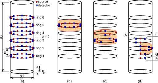 Three different focus regions were chosen to demonstrate the focusing capability. Region A consists of the voxels in the cylinder slice given by , region B is another slice defined by , and region C is the half-cylinder slice and . The adaptation was performed on a finite element mesh with approximately 30,000 elements. Looking at the outcome of the adaptation procedure, one notices that the algorithm tends to concentrate the final sources and optodes near the focus regions, which is desired because the sensitivity is usually higher toward the optodes. The result of adapting to the uppermost focus region in Fig. 1 could also have been suggested intuitively. On the other hand, the best configuration in Fig. 1 is symmetric around the cylinder’s axis but asymmetric to its midplane. We also compared the geometric averaging method to the original formulation published in Ref. 16. The result of the adaptation using the arithmetic averaging is to a large extent equivalent to the geometric averaging method, and so we indicate only the differences in Fig. 1. Focusing to regions A and B resulted in exactly the same optode set. Only when focusing on the half-cylinder slice, two detectors changed their location. Their position in Fig. 1 has been labeled G for the geometric and A for the original arithmetic averaging. This is an expected result, as the geometric averaging method replaces only one of the sums by a product and thus there should not be a dramatic difference in the best optode configuration. From these outcomes, one can conclude that both the geometric and the arithmetic adaptation methods result in optode configurations that are meaningful and comprehensible. Figures 2, 2, 2 show the rank of the optodes, i.e., the iteration in which they were removed from the pool of feasible optodes for the geometric averaging method. The lighter the color, the longer the optode remains in the feasible pool. There is a general tendency to remove optodes far from the focus region early from the adaptation process, as can be seen by looking at the lower optode rings in Fig. 2 or at rings 1 and 6 in Fig. 2. However, this is not the case anymore when the region of interest is set to the half-cylinder slice, where the first optodes to be removed are the ones on ring 2 opposite the focus region. There are also optodes on ring 5 that stay longer in the feasible pool. This can be explained by the fact that off-plane information could improve the resolution in the direction of the cylinder axis. Fig. 2The rank of the removed optodes using the geometrical weighting encoded in color for three different focus regions (sketched in orange). Optodes drawn in black or red were eliminated early during the adaptation process, while those in yellow and white remained longer in the pool. The final set of optodes has been omitted. (Color online only.)  4.2.Comparison of Reconstructed ImagesTo provide evidence that the adapted arrangements improve reconstruction results, simple symmetrical optode arrangements were compared to the results of the adaptation algorithms. To quantify the reconstructed images in an objective manner, a reconstruction with the full set of optodes was used as gold standard, as this is the best reconstruction one can achieve under the given circumstances. First, four fluorescent inclusions with a diameter of were placed inside the focus region B. Every second source and detector optode on the rings 3 and 4 were chosen as an intuitive arrangement. This configuration resulted in a relative reconstruction error of 46% compared to the reconstruction with all optodes. The reconstruction with the best set of optodes for region B (which is the same for both adaptation methods) yielded a relative error of 42%. For the second test case, a single sphere was placed inside focus region C. The relative error of the intuitive arrangement—which was all optodes on ring 2—to the best possible reconstruction was 25.6%. Using the geometrically weighted adapted optode set resulted in a relative error of 16.9%. The best configuration using the adaptation routine with arithmetic averaging yielded an error of 17.4%. For the focus region A, the adapted optode configurations are identical to the intuitive one. As an objective quality measure for the sensitivity matrix of the adapted optodes, its singular values or its condition number can be used. The largest and smallest singular values together with the ratio between them can be found in Table 2 . The full optode configuration has a rather high ratio of and is thus rather ill-conditioned. The focused designs show a singular value (SV) ratio that is reduced by a factor of to . This is exactly what is intended by the redundancy minimization algorithm, as the removal of nonorthogonal rows from the sensitivity matrix improves conditioning. As the adaptation method with geometric and arithmetic averaging resulted in nearly optimal optode configurations, the difference in singular values when focusing on region C is rather small. Table 2Singular value (SV) analysis for the full sensitivity matrix and the adapted configurations with focusing on different regions. The table lists the largest and smallest singular values as well as the ratio between them (the condition number), which is a measure of stability for matrix inversion.
4.3.RobustnessThe robustness of the adaptation method was tested by a Monte Carlo simulation. First, the best adapted configurations using either the arithmetic or the geometric averaging were defined as reference sets. In each run of the Monte Carlo simulation, the optodes in the initial pool were shifted randomly up to along the axis and the cylinder perimeter (which is a shift of 10% of the distance between two optodes in direction and 15% along the perimeter), after which the adaptation procedure was used on these shifted optodes. Table 3 lists the number of 50 Monte Carlo trials for which the adapted set did not differ by more than four optodes from the reference set with an unshifted initial optode pool. Table 3Number of Monte Carlo trials with shifted initial optode positions that resulted in an adapted optode set that did not differ from the reference set by more than nmiss (cumulated).
The shifting of the optodes has obviously no influence when focusing on region A, as both averaging methods are able to return the best solution in every Monte Carlo trial. In the other two cases where the best solution is not so obvious, the stability is decreased a bit. This is especially true when focusing on region B. One reason is that in this setup, the best set of optodes can be rotated around the cylinder’s axis or mirrored at the -plane, and the resultant configuration should be equivalent to the reference solution with respect to redundancy in measurement data. For Fig. 3 , the frequency of every optode in the final set was counted, coded in the marker size, and drawn on the cylinder surface. The bigger the optode circle (source) or square (detector) is drawn, the more often this optode will be in the outcome of the adaptation process and the more stable it is. The reference result for which the initial pool of optodes was left unshifted is marked with an . It is well visible that the optodes are always placed near the focus region. Fig. 3Stability of the adaptation result using geometric averaging for focus regions B (a) and C (b). Sources are drawn as circles, detectors as squares. The marker size is proportional to the stability of the optode. Optodes from the reference set (unshifted initial pool of optodes) are marked with x.  Last, Table 4 shows the mean value and standard deviation of the quality measure from Eqs. 27, 28 for the best and worst source and detector optode. The standard deviation is quite small, which indicates that even if the adaptation method does not find the optodes from the reference set, the resultant optodes still have a high quality, i.e., their measurements exhibit a small redundancy. Table 4Mean and standard deviation of the quality measure for the best and worst source and detector optodes over all Monte Carlo runs.
4.4.Off-Focus Signal SuppressionFigure 4 shows example reconstructions based on artificial measurement data for three spherical perturbations with a diameter of , using the three different focusing strategies together with geometric averaging. The exact locations of the perturbations are shown in Fig. 4. The optical properties are the same as listed in Table 1. The synthetic data was generated using a finer finite element mesh, and 5% noise was added. It can be noticed that every configuration is able to suppress the signal from outside its focus region quite effectively. The reconstruction is best for the lower sphere because the optode configuration was adapted to a smaller focus volume there. Fig. 4Reconstruction examples for differently focused optode setups. (a) The simulation model used to generate artificial measurement data for all optode setups. The spherical perturbations have a diameter of . The six dotted horizontal lines mark the location of the optode rings. The other figures show reconstructions when focusing on region A (b), region B (c), or region C (d) with the optimal setup gained with the geometric averaging method.  5.DiscussionThe location of the sensors and detectors is a critical design parameter for FDOT hardware. A configuration determines the sensitivity of the measurements in a given region and also the obtainable resolution. The method presented in this paper is based on a simulation model and can thus be used prior to building hardware. Comparisons of different hardware configurations for fluorescence tomography that we are aware of were previously reported by Graves 2 and Lasser 3 Their approaches were based on a singular value (SV) analysis of the so-called weight matrix. This matrix is essentially the sensitivity matrix used in this paper, but was obtained using the normalized Born approximation.19 In contrast to the previous methods, the adaptation algorithm used herein operates on the complete derivative of the diffusion approximation 7. Therefore, also the change of the excitation field due to a perturbation in the fluorophore distribution is considered, which is neglected in commonly used first-order Born approximations. The SV analysis implemented by Graves and Lasser requires a singular value decomposition (SVD) of the sensitivity matrix. This demands a large amount of computation time. As an example, the calculation of a single SVD for a matrix of size takes about on a dual-core processor. Therefore, the SV optimization is limited to 2-D applications or to rather simple 3-D geometries, which can be modeled with fewer finite elements. The redundancy reduction algorithm does not suffer from these limitations, as it needs to compute only inner products of rows of the sensitivity matrix. The matrix is built up efficiently using an implicit function formulation that requires one additional finite element solution per optode only. Furthermore, both the assembly of the sensitivity matrix as well as the calculation of the inner products can be parallelized with moderate effort (the basic principle can be found in Ref. 20, for example), which allows accelerating the method even more. The algorithm we implemented starts with a complete optode arrangement and iteratively discards the one optode having the lowest quality measure. Unfortunately, the algorithm cannot determine in the current step whether it would be advantageous later if the worst optode was kept and another one was dismissed from the pool instead. Thus, the drawback of this simple top-down strategy is that it cannot guarantee to find the global minimum. However, a full search is an nondeterministic polynomial time (NP) problem and would require the computation of around different configurations for the rather simple geometry demonstrated earlier. This is computationally not feasible. A viable alternative could be the implementation of stochastic methods that have a long tradition in numerical optimization. A recent promising approach involves formulating this problem as a distributed control problem with sparsity constraints,21, 22 which computes an “optode field” that is nonzero only at discrete points. These could be taken as optimal locations where optodes should be placed. In addition, the solution would indicate the optimal strength of the sources as well. A great advantage of the redundancy minimization is that it provides a quality measure for every single optode rather than comparing complete configurations, as is the case in SV analysis. This offers the possibility to choose a superior configuration first, which could even be obtained with a completely different method, and to adapt the arrangement further through the removal of optodes exhibiting a poor quality measure. To our knowledge, the possibility of choosing an optode configuration such that the reconstruction is focused on an a priori given region inside the tissue has not been investigated for fluorescence tomography before. Similar strategies have been reported for other diffusion-limited imaging modalities such as seismic tomography16 and magnetic induction tomography.23 The effect of focusing on the reconstruction is demonstrated in Figure 4. The best reconstruction result is obtained when the optode configuration is adapted to a small volume around the field of view, which is demonstrated in Fig. 4. In all three reconstructions, the concentration changes outside the focus region are suppressed very well. This feature might prove advantageous in certain cases—for example, if the autofluorescence signal from other organs needs to be damped. In Sec. 3.2, we attempted to link the redundancy measure to entropy and mutual information, respectively. The three quality criteria given in Eqs. 32, 33, 24 are very similar in their structure, although not equal. The mutual information criterion operates on the full covariance matrix, while the redundancy criteria use its diagonal part only. The MI optimization is computationally expensive due to the need for matrix decompositions, matrix inversions, and the calculation of the determinant. The redundancy reduction is much more efficient, as it mainly depends on the calculation of inner products of matrix rows. However, the decrease in numerical effort goes hand in hand with the neglect of the off-diagonal matrix entries. In this paper, one of the most simple stopping criteria, the final number of sources and detectors, was chosen. It is worth mentioning that the algorithm is flexible enough to include more elaborate criteria easily. For example, it could be desirable to specify the minimum required resolution or the minimum contrast-to-noise ratio. In further work, the feasibility of dynamic stopping criteria will also be investigated. The principle is to calculate an initial image quality criterion (e.g., the resolution) and then again iteratively remove optodes from the feasible pool. As soon as the image quality decreases significantly, the procedure is stopped. 6.ConclusionWe have presented an algorithm to adaptively remove sensor and detector locations for fluorescence diffusion optical tomography. The possibility to bias the resultant design to be sensitive in a given area was demonstrated. In contrast to previously reported algorithms, the current formulation has a strong connection to entropy optimization. AcknowledgmentsThis work was supported by Project F3207-N18 granted by the Austrian Science Fund. The authors want to thank the referees for their helpful comments, which led to a significant improvement in the revision of this paper. ReferencesJ. Mobley and
T. Vo-Dinh,
“Optical properties of tissue,”
Biomedical Photonics Handbook, 2/1
–2/75 CRC Press, Boca Raton, FL
(2003). Google Scholar
E. E. Graves,
J. P. Culver,
J. Ripoll,
R. Weissleder, and
V. Ntziachristos,
“Singular-value analysis and optimization of experimental parameters in fluorescence molecular tomography,”
J. Opt. Soc. Am. A, 21 231
–241
(2004). https://doi.org/10.1364/JOSAA.21.000231 0740-3232 Google Scholar
T. Lasser and
V. Ntziachristos,
“Optimization of 360° projection fluorescence molecular tomography,”
Med. Image Anal., 11 389
–399
(2007). https://doi.org/10.1016/j.media.2007.04.003 1361-8415 Google Scholar
S. R. Arridge,
“Optical tomography in medical imaging,”
Inverse Probl., 15 R41
–R93
(1999). https://doi.org/10.1088/0266-5611/15/2/022 0266-5611 Google Scholar
A. Joshi,
“Adaptive finite element methods for fluorescence enhanced optical tomography,”
Texas A&M University,
(2005). Google Scholar
R. B. Schulz,
J. Peter,
W. Semmler,
C. D’Andrea,
G. Valentini, and
R. Cubeddu,
“Comparison of noncontact and fiber-based fluorescence-mediated tomography,”
Opt. Lett., 31 769
–771
(2006). https://doi.org/10.1364/OL.31.000769 0146-9592 Google Scholar
E. Zeidler, Applied Functional Analysis: Main Principles and Applications, 109 Springer-Verlag, New York
(1995). Google Scholar
S. F. Gull and
J. Skilling,
“Maximum entropy method in image processing,”
IEE Proc. F, Commun. Radar Signal Process., 131 646
–659
(1984). 0143-7070 Google Scholar
A. J. Mwambela,
Ø. Isaksen, and
G. A. Johansen,
“The use of entropic thresholding methods in reconstruction of capacitance tomography data,”
Chem. Eng. Sci., 52 2149
–2159
(1997). https://doi.org/10.1016/S0009-2509(97)00041-9 0009-2509 Google Scholar
N. V. Denisova,
“Maximum-entropy-based tomography for gas and plasma diagnostics,”
J. Phys. D: Appl. Phys., 31 1888
–1895
(1998). https://doi.org/10.1088/0022-3727/31/15/018 0022-3727 Google Scholar
A. Mohammad-Djafari and
G. Demoment,
“Maximum entropy image reconstruction in x-ray and diffraction tomography,”
IEEE Trans. Med. Imaging, 7 345
–354
(1988). https://doi.org/10.1109/42.14518 0278-0062 Google Scholar
M. K. Nguyen and
A. Mohammad-Djafari,
“Bayesian approach with the maximum entropy principle in image reconstruction from microwave scattered field data,”
IEEE Trans. Med. Imaging, 13 254
–262
(1994). https://doi.org/10.1109/42.293918 0278-0062 Google Scholar
B. A. Ardekani,
M. Braun,
B. F. Hutton,
I. Kanno, and
H. Iida,
“Minimum cross-entropy reconstruction of pet images using prior anatomical information,”
Phys. Med. Biol., 41 2497
–2517
(1996). https://doi.org/10.1088/0031-9155/41/11/018 0031-9155 Google Scholar
N. A. Ahmed and
D. V. Gokhale,
“Entropy expressions and their estimators for multivariate distributions,”
IEEE Trans. Inf. Theory, 35 688
–692
(1989). https://doi.org/10.1109/18.30996 0018-9448 Google Scholar
S. Puntanen and
G. P. H. Styan,
“Schur complements in statistics and probability,”
The Schur Complement and Its Applications (Numerical Methods and Algorithms), 163
–226 Springer, New York
(2005). Google Scholar
A. Curtis,
A. Michelini,
D. Leslie, and
A. Lomax,
“A deterministic algorithm for experimental design applied to tomographic and microseismic monitoring surveys,”
Geophys. J. Int., 157 595
–606
(2004). https://doi.org/10.1111/j.1365-246X.2004.02114.x 0956-540X Google Scholar
G. Alexandrakis,
F. R. Rannou, and
A. F. Chatziioannou,
“Tomographic bioluminescence imaging by use of a combined optical-pet (opet) system: a computer simulation feasibility study,”
Phys. Med. Biol., 50 4225
–4241
(2005). https://doi.org/10.1088/0031-9155/50/17/021 0031-9155 Google Scholar
M. Keijzer,
W. M. Star, and
P. R. M. Storchi,
“Optical diffusion in layered media,”
Appl. Opt., 27 1820
–1824
(1988). https://doi.org/10.1364/AO.27.001820 0003-6935 Google Scholar
V. Ntziachristos and
R. Weissleder,
“Experimental three-dimensional fluorescence reconstruction of diffuse media by use of a normalized born approximation,”
Opt. Lett., 26 893
–895
(2001). https://doi.org/10.1364/OL.26.000893 0146-9592 Google Scholar
G. Haase,
M. Kuhn, and
U. Langer,
“Parallel multigrid 3D Maxwell solvers,”
Parallel Comput., 27 761
–775
(2001). https://doi.org/10.1016/S0167-8191(00)00106-X 0167-8191 Google Scholar
G. Stadler,
“Elliptic optimal control problems with -control cost and applications for the placement of control devices,”
Comput. Optim. Appl., 44 159
–181
(2009). https://doi.org/10.1007/s10589-007-9150-9 0926-6003 Google Scholar
C. Clason and
K. Kunisch,
“A duality-based approach to elliptic control problems in non-reflexive Banach spaces,”
ESAIM Control, Optimisation and Calculus of Variations, 2009). Google Scholar
D. Gürsoy and
H. Scharfetter,
“Optimum receiver array design for magnetic induction tomography,”
IEEE Trans. Biomed. Eng., 56 1435
–1441
(2009). https://doi.org/10.1109/TBME.2009.2013936 0018-9294 Google Scholar
|
|||||||||||||||||||||||||||||||||||||||||||||||||||||||||||||||||||||||||||||||||||||||||||||||||||||||||||||||||||||||||||||||||||||||||||||||||||||||


