|
|
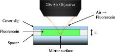
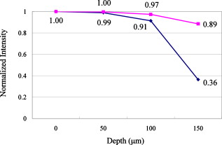
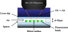
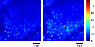
1.IntroductionTwo-photon excitation fluorescence microscopy has millimeter scale penetration depth in biological specimens.1, 2 However, the refractive index inhomogeneity in these samples often distorts the wavefront of the excitation light, resulting in a broader focal point spread function and lower two-photon excitation efficiency. With an adaptive optics system, this wavefront distortion can be compensated, and image resolution and signal level can be preserved at greater imaging depth. The adaptive optics approach was first developed in fields such as astronomy3 and ophthalmology.4 In microscopy, significant progress has been made in confocal systems,5, 6 and adaptive optics has also been applied to nonlinear microscopies such as two-photon excitation microscopy,7, 8 harmonic generation microscopy,9, 10 and coherent anti-stokes Raman scattering (CARS) microscopy.11 The different implementations of adaptive optics to nonlinear microscopy can be roughly classified into two approaches: feedback via two-photon excited fluorescence light, or feedback via reflected excitation light. Most fluorescence light feedback systems are based on maximizing signal strength, for example, by varying the shape of the deformable mirror via genetic algorithms,12, 13 or image-based algorithms.14 In addition, the choice of performance parameters for feedback control using genetic algorithms (e.g., brightness, contrast, and resolution) have been investigated.15 As an alternative approach, a differential aberration imaging technique has been demonstrated by rejecting out-of-focus fluorescence background signals by using a defocused image.16 For feedback control using reflected excitation light, most implementations utilize the coherent nature of the reflected light and incorporate a wavefront sensor component. A major challenge in applying wavefront sensing in nonlinear microscopes with inherent 3-D resolution is to select the reflected light signal preferentially from the focal plane of interest but not throughout the optical path of the excitation light. In one approach, Feierabend, Rueckel, and Denk,17 and Rueckel, Mack-Bucher, and Denk18 used a coherence-gated wavefront sensing method. This approach utilizes the low temporal coherence properties of femtosecond laser pulses. The reflected light signal from the focal plane is selected interferometically via a modified Michelson interferometer, and the wavefront distortion is quantified using a shear interferometer. In this work, we demonstrate an alternative method for adaptive correction in two-photon microscopy via reflected light feedback utilizing the confocal principle for depth selection. This approach simplifies the optics in the wavefront detection light path and reduces the potential of inducing additional aberrations. Further, we utilize a Shack-Hartmann wavefront sensor that allows the wavefront distortion to be monitored by acquiring a single image, improving the bandwidth of the adaptive optics feedback loop. 2.Methods and Experimental SetupThis two-photon microscope with adaptive optics compensation was constructed by modifying an existing system, as previously described.2 The major additional components consist of a large dynamic range deformable mirror, a Shack-Hartmann wavefront sensor, and a confocal light path for reflected light detection. 2.1.Large Dynamic Range Deformable MirrorThe deformable mirror (Mirao52d, Imagine Optic, Orsay, France) includes a silver-coated reflective membrane coupled with 52 miniature voice-coil-type actuators. The diameter of its pupil is and it has a bandwidth. The maximum wavefront amplitude that can be generated is with voltage range. An important feature of this deformable mirror is its large dynamic range. It can generate mimic Zernike modes up to the fourth order and partially up to the sixth order. 2.2.Detection of the Wavefront Distortion with a Shack-Hartmann Wavefront SensorThe Shack-Hartmann wavefront sensor (HASO32, Imagine Optic, Orsay, France) consists of a lenslet array and a charge-coupled device (CCD) sensor. It has lenslets within a rectangular aperture. Its bandwidth is . With an incident plane wave, an array of foci produces a rectilinear grid defined by the lenslet dimension. However, if the incoming wavefront is distorted, the foci are displaced from the grid location. By measuring the distance of the displacement using a CCD camera, the slope of the local wavefront can be calculated and the whole wavefront can be constructed. The advantage of the Shack-Hartmann sensor is its ability to rapidly quantify wavefront aberration with a single image. 2.3.Application Confocal Detection to Select Reflected Light Signals from the Focal PlaneOnly the aberration information of light from the focal region of the objective is relevant for optimizing two-photon excitation. However, a reflected light signal is not only produced at the focal plane, but also from out-of-focal regions. The signal from out-of-focal regions needs to be eliminated, and we accomplished it by setting up a confocal detection light path. The confocal pinhole passes the signal originating from the focal region of the objective while blocking the out-of-focus light at the confocal pinhole. The depth selectivity, axial resolution, should be optimized by selecting a small pinhole.19, 20 However, this requirement must be traded off against the fact that the pinhole also acts as a spatial filter. A very small pinhole will filter out all higher spatial frequency information of the distorted wavefront needed for adaptive correction. These two conflicting requirements must be balanced in our system. The optimization of the pinhole size is discussed in the next section. 2.4.Overall Instrument ConfigurationFigure 1 describes the general experimental setup. The laser source was a Ti-sapphire (Ti-Sa) laser (Tsunami, Spectra-Physics, Mountain View, California) pumped by a frequency-doubled Nd:YVO4 laser (Millennia V, Spectra-Physics, Mountain View, California). The excitation light was reflected by the deformable mirror (Mirao52d, Imagine Optic, Orsay, France), positioned at a conjugate plane of the back aperture of the microscope objective, toward the excitation optical path of a typical two-photon laser scanning microscopy.2 The emission fluorescence signal passing a short-pass dichroic mirror and a short-pass barrier filter (650dcxxr and E700SP, Chroma Technology, Rockingham, Vermont) was incident on a photomultiplier detector (R7400P, Hamamatsu, Bridgewater, New Jersey) and the associated single-photon counting circuitry. The scattered light signal was reflected by the dichroic scanner, descanned by passing through the scanning mirrors, and directed toward the wavefront camera (HASO32, Imagine Optic, Orsay, France). The wavefront camera was also positioned at a conjugate plane of the microscope objective back aperture. Before the wavefront camera, a confocal pinhole (P150S, Thorlabs, Newton, New Jersey) was positioned at a plane conjugated to the microscope focal plane selecting a depth-resolved reflected light signal. Fig. 1System configuration. The components used are a Ti-sapphire (Ti-Sa) laser, plano-convex lens L1 (focal length , KPX082AR.16, Newport) L2 (f , KPX106AR.16, Newport), L3 (f , KPX094AR.16, Newport), L5 (f , KPX106AR.16, Newport), L6 (f , KPX115AR.16, Newport), L7 (f , KPX082AR.16, Newport), L8 (f , 444232, Zeiss), L10 (f , KPX097AR.16, Newport), L11 (f , KPX106AR.16, Newport), L13 (f , KPX094AR.16, Newport), silver-coated mirrors (10D20ER.2, Newport), beamsplitter (10BC17MB.2, Newport), deformable mirror (Mirao52d, Imagine Optics), scanning mirrors (6350, Cambridge Technology), short-pass dichroic mirror (650dcxxr, Chroma Technology), objective lens (Fluar, , Zeiss), photomultiplier detector (R7400P, Hamamatsu), pinhole (P150S, Thorlabs), and wavefront camera (HASO32, Imagine Optics). 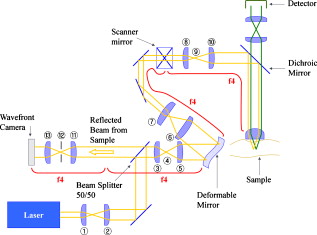 As described before, a small pinhole is necessary for good axial resolution. However, the pinhole also should be sufficiently large to pass the spatial frequency information contained in the distorted wavefront. We set the minimum pinhole size based on the highest spatial frequency that the deformable mirror can generate, because higher order distortion cannot be corrected in any case. The distances between the two actuators on the deformable mirror are , corresponding to a minimum spatial period of . Fourier transform of this spatial period gives a maximum spatial frequency that needs to pass through the wavefront detection light path. We determined that a confocal aperture with diameter no less than placed at plane 12 of Fig. 1 would transmit all the relevant aberration information. However, we chose to use a -diam pinhole to provide some additional margin of error. It is necessary to examine what axial resolution is afforded by this -diam pinhole. Accounting for the magnification of the intermediate lenses, the pinhole at plane 12 corresponds to an effective aperture of radius at plane 9 of Fig. 1. At plane 9, the axial resolution is related to the aperture size by Eq. 1:21 where is the radius of the aperture , is for an oil-immersion objective lens (Fluar, , Zeiss, Thornwood, New York), NA is the numerical aperture of the objective lens, is the index of refraction of the medium, and is the magnification. Since the focal length of lens 10 is , the effective magnification is 30.3. This results in an axial resolution of about . This resolution is more than sufficient, because the back aperture of the objective is underfilled corresponding to an effective axial resolution of , discussed later in Sec. 3.2.By measuring the wavefront distortion, the wavefront camera provided feedback signals to the deformable mirror. The deformable mirror generated predistortion to the plane wave that countered the distortion induced by the sample. The predistortion from the deformable mirror and the distortion from the sample were cancelled out to produce a more ideal point spread function at the focal point. It should be noticed that the light that was detected by the wavefront camera passed the deformable mirror twice, while the actual incoming excitation light to a sample passed the deformable mirror once. Under the assumption that the specimen is highly scattering, this is the appropriate optical configuration, since the detected light also was aberrated twice by the sample in the reflected light mode. Therefore, with closed-loop control, the adaptive optics compensation worked with the predistorted excitation light before the sample, producing a flat wavefront at the wavefront camera after the feedback system reaches steady state. Figures 2 and 3 show representative wavefronts and aberration coefficients before and after adaptive optics compensation. The wavefront sensor provides the deformable mirror with the feedback signal, satisfying four-fold of Nyquist–Shannon sampling criterion. Therefore, the adaptive optics system can correct the wavefront up to the maximum capability of the deformable mirror, which is under rms error according to its specification. Fig. 2Wavefront change after AO compensation. The sample is a mouse heart (described in Sec. 3.4) and imaged at depth. (a) Distorted wavefront without the compensation. (b) Wavefront after AO compensation.  Fig. 3Third-order aberration coefficient change after AO compensation. (a) Uncompensated coefficients corresponding to Fig. 2. The axis represents Zernike coefficients; 4 is , 5 is , 6 is , 7 is , and 8 is . The error of the wavefront measurement is less than . (b) Compensated coefficients. 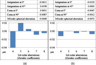 It should also be noted that our method holds only when the sample is highly scattering, which is often (but not always) the case in biological samples. For a more reflective sample, the measured wavefront is dependent on whether the aberrations generated by the sample are odd (asymmetric) or even (symmetric), which was extensively discussed in Refs. 22, 23, 24. For a reflective sample with the odd aberrations, this system configuration gives incorrect wavefront measurements. In our system configuration, there are losses of excitation laser power and reflected light signal due to the use of the beamsplitter. The losses can be avoided by using a polarizing beamsplitter followed by a quarter-wave plate.8 This configuration reflects 100% of the excitation laser power instead of 50% in the absence of multiple scattering. 3.Experiment and ResultTo thoroughly quantify the performance of our adaptive optics system, we have devised a series of experiments using artificial and biological specimens. Two artificial specimens with large aberrations were prepared and used to evaluate our adaptive optics system in terms of minimizing signal loss and optimizing image resolution loss. Also, the performance of this adaptive optics system was evaluated in three typical biological tissue specimens: mouse tongue muscle, heart muscle, and brain slice. 3.1.Signal Loss Due to Aberrations as a Function of Imaging DepthThis experiment was designed to measure the signal loss due to aberration as a function of imaging depth and the compensatory performance of the adaptive optics system. A air objective lens (Fluar, , Zeiss, Thornwood, New York) was intentionally used to image into aqueous fluorescein samples with varying thicknesses: 50, 100, and (Fig 4 ). A mirror (10D20ER.2, Newport, Irvine, California) was placed at the bottom of the specimen to enhance reflected light signals. A femtosecond pulsed laser (Tsunami, Spectra-Physics, Mountain View, California) was used to provide excitation light. The two-photon excitation focal volume was placed just above the mirror surface within . The refractive index mismatch between the air objective and the aqueous specimen resulted in the generation of significant aberration, especially spherical aberration.25, 26 As the focus went deeper, the signal loss became higher. The signal loss was measured with a normal two-photon excitation fluorescence microscope with and without the adaptive optics compensation, and the two signal losses were compared. Figure 5 shows the result of the fluorescein emission signal loss experiment. The uncompensated signal is the blue line and the compensated signal is the pink line. The uncompensated signal decreased with increasing focus depth. However, with adaptive optics compensation, the emission signal remained almost constant. The signal improvement was 1% at , 7% at , and 147% at . At , the maximum Zernike coefficient of the uncompensated aberration among the third-order aberrations was , but it became with the adaptive optics compensation. The Zernike coefficient for spherical aberration was reduced from . The maximum aberration was astigmatism instead of the spherical aberration, and it may be caused either by slight misalignment of the lenses or by slight bending of the dichroic mirror, which is common in some microscope dichroic mirror holders.27, 28 In addition, the excitation laser source was linearly polarized in front of the sample instead of circularly polarized, and it is known that scattering depends on the polarization direction. Therefore, linearly polarized excitation light may generate erroneous astigmatism.18 3.2.Point Spread Function Degradation Due to Aberrations as a Function of Imaging DepthIn this experiment, we tried to quantify point spread function degradation due to aberrations as a function of imaging depth and the compensatory performance of the adaptive optics system. A oil immersion objective lens (Fluar, , Zeiss, Thornwood, New York) was used to image -diam fluorescence beads (F8803, Invitrogen, Eugene, Oregon) deposited on a mirror through an air gap of (Fig. 6 ). The mirror was used to enhance the reflected light signal. The excitation wavelength was . Spherical aberration was again generated due to index mismatch between the oil objective and the air specimen. The point spread function was measured with a normal two-photon excitation fluorescence microscope with and without the adaptive optics system. Figure 7 shows the effect of aberration on PSF laterally and axially. The blue bar shows the uncompensated resolution and the pink bar shows the compensated resolution. Clearly, when the air gap thickness is zero, no compensation is necessary. At air gap, lateral resolution was improved by 12% and axial resolution was improved by 38%. Lateral resolution is proportional to and axial resolution is proportional to , so it is a reasonable result that axial resolution was affected more than lateral resolution with the adaptive optics compensation. The Zernike coefficient of the uncompensated maximum aberration had been , but it became with compensation. The Zernike coefficient for spherical aberration became . Here the reason that the spherical aberration was not the maximum value among the third-order aberrations may be again due to reasons cited in the previous section. Fig. 7Resolution change after AO compensation. (a) Lateral resolution change. (b) Axial resolution change.  Furthermore, we should note that the lateral and axial resolutions were larger than the values of diffraction-limited resolutions. This was because the objective lens was underfilled by the excitation light. As we mentioned with the system configuration, the deformable mirror gives the same compensation to the input beam and the outgoing beam from the sample. The two beams should be located exactly at the same area on the deformable mirror, so their beam sizes should be the same and the objective was just filled with the excitation light. However, because of the Gaussian characteristic of the laser beam, the objective lens was practically underfilled and the lateral and axial resolutions became larger. According to the experimental result, the effective NA of the objective was about 0.55 in our experimental setup, although its theoretical NA is 1.3, which is valid only when immersion oil is present under the objective lens until a cover slip, and a sample is then just below the cover slip in a refractive index of 1.5. This current limitation can be removed by utilizing a top-hat wavefront shaper or modifying the adaptive optics feedback algorithm to ignore information from the peripheral region of the wavefront sensor. 3.3.Mouse Tongue Muscle Imaging Using Adaptive-Optics-Compensated Two-Photon MicroscopyMouse tongue musculature was visualized based on both endogenous fluorescence and second harmonic generation. A whole tongue excised from a female C57BL/6 mouse ( old) was fixed in phosphate buffered saline (PBS, pH 7.4) containing 2.5% glutaraldehyde for about a day. The fixed tongue tissue was then immersed in PBS for , rinsed with the same buffer excessively, and finally embedded in paraffin without a cover slip. The wavelength of the excitation light was set to . The objective lens was a oil-immersion objective lens (Fluar, , Zeiss, Thornwood, New York). The emission signal was filtered by a green filter (535/40, Chroma Technology, Rockingham, Vermont). The field size was with , and the dwell time was . As representative images, Fig. 8 shows mouse tongue muscle images at depth with and without the adaptive optics compensation. The left image is the uncompensated image, and the right one is the compensated image, and they were processed with background rejection. The threshold for each image was set to three times the intensity level measured in regions outside objects of interest (e.g., blood vessels in the mouse heart or the neurons in the mouse brain). In principle, the bandwidths of the wavefront camera and the deformable mirror are about and , respectively. However, the current feedback algorithm takes significant CPU resources, and it leads to a compensation time of . Therefore, the algorithm is the bottleneck for the bandwidth of the whole compensation process, and it is far from practical for pixel-by-pixel correction over the whole image. Instead, with the assumption that the optical paths are similar over the scanned area of the image, adaptive optics compensation was performed only at the center pixel of the image, and the rest of the image was acquired with the same deformable mirror shape setting.29 In future studies, it would be interesting to determine the optimal number of pixels that should be corrected per image given the tradeoff between imaging speed and tissue heterogeneity. It would also be interesting to improve imaging speed by developing faster, more efficient feedback algorithm or by utilizing higher performance computer hardware. The compensated image shows higher signal strength than the uncompensated one. To compare the signal intensity of two images, intensity distributions for all pixels were calculated. Figures 9, 9, 9, 9 show the histograms for the intensity distributions before and after the compensation. It was shown that the number of brighter pixels increased and the number of darker pixels decreased for all imaging depths after the compensation, which means the in-focus fluorescence signals were improved, while the out-of-focus fluorescence signals were suppressed. To find the improvement trend according to imaging depth, mean photon counts were calculated with background rejection. Figure 9 shows the percentage improvement from the mean photon counts according to imaging depth. The percentage improvement shows that at greater imaging depth, the improvement becomes larger, so the improvement for 90 to 100% intensity pixels was 38.1% at depth. Figure 9 shows the increment of mean photon count. In terms of the increment of photon count, the result at depth shows the greatest improvement than at greater depths. At shallow depths, there is not much to compensate, and at greater depths the overall signal is significantly lower due to scattering attenuation of both excitation and emission photons.30 Figure 9 shows the percentage improvement based on each pixel at depth, calculated from Fig 8. Comparing the degree of improvement on the center versus the edge, no major difference is observed. From all over the region where the fluorescence signal is generated, the improvement seems quite uniform. This might be because the aberration from the optical system is much larger than the aberration from the sample. Fig. 9Signal improvement after AO compensation. (a) through (d) show histograms for the number of pixels according to their intensity; axis represents intensity of the pixels. For example, 10 means that the pixels have 0 to 10% intensity of the maximum in the whole image, and 100 means 90 to 100% intensity pixels. The axis represents the number of pixels in the intensity range. The blue bars show the number of pixels before the compensation, and red bars show the result after compensation. Each histogram was normalized to itself. (a) shows the distribution at depth, (b) at , (c) at , and (d) at imaging depth. (e) Percentage improvement according to imaging depth. The red line shows the improvement with background rejection (only the fluorescent area was calculated), and the blue line shows the improvement only with 90 to 100% intensity pixels. (f) Increment of mean photon count. Red and blue lines show the same datasets as (e). (g) Percentage improvement based on each pixel. Any pixel with more than two-fold improvement, that comes from a mismatch of the uncompensated and compensated image, is saturated to a red color. The background is set to for visualization purposes. (Color online only.)  3.4.Mouse Heart Muscle Imaging Using Adaptive-Optics-Compensated Two-Photon MicroscopyAs a second example, we imaged mouse heart muscular structures with nuclei based on endogenous fluorescence, second harmonic generation, and exogenous labeling. Through tail-vein injection (in conjunction with an overdose of anesthetics), nuclei are labeled with Hoechst, while the extracellular matrix around the cells are labeled with Texas-Red maleimide. After staining, the heart was excised and was fixed in 4% paraformaldehyde and embedded in paraffin without a cover slip after some histological processing. The wavelength of the excitation light was . The objective lens was a oil-immersion objective lens (Fluar, , Zeiss, Thornwood, New York). The emission signal was filtered by a green filter (535/40, Chroma Technology, Rockingham, Vermont). The field size was with , and the dwell time was . Figure 10 shows representative images of mouse heart at depth with and without adaptive optics compensation. The left image is the uncompensated image, and the right one is the compensated image. As in the mouse tongue experiment, adaptive correction was only performed at the center pixel of the image, and the same deformable mirror shape was held constant throughout the whole image. To compare the signal intensity of the two images, the intensity distributions for all pixels were calculated again. Figures 11, 11, 11, 11 show the histograms for the intensity distributions before and after the compensation. The same trend was shown as the mouse tongue result; the number of brighter pixels increased, and the number of darker pixels became less for all imaging depths after the compensation. To find the improvement trend according to imaging depth, mean photon counts were calculated with background rejection. Figure 11 shows the percentage improvement from the mean photon counts according to imaging depth. The percentage improvement shows that as the imaging plane went deeper, the improvement became larger in general. The maximum improvement of the 90 to 100% intensity pixels was 123% at depth. Fig. 11Signal improvement after AO compensation. (a) through (d) show histograms for the number of pixels according to their intensity; the axis represents the intensity of pixels the same as in Fig. 9, except 100 (100 means 40 to 100% intensity pixels in the image). The axis represents the number of pixels in the intensity range. The blue bars show the number of pixels before the compensation, and the red bars show the result after compensation. Each histogram was normalized to itself. (a) shows the distribution at depth, (b) at , (c) at , and (d) at imaging depth. (e) Percentage improvement according to imaging depth. The red line shows the improvement with background rejection (only the fluorescent area was calculated), and the blue line shows the improvement only with 90 to 100% intensity pixels. (Color online only.)  In terms of the increment of photon count, the result at depth showed the greatest increase due to the generally higher signal level. At greater depths, scattering of excitation and emission photons again dominated, and the improvement due to using adaptive optics became less significant. In terms of improvement on the center compared to the edge, it seemed to be uniform, similar to the mouse tongue result. 3.5.Neuronal Imaging in Mouse Brain Slices Using Adaptive-Optics-Compensated Two-Photon MicroscopyBoth muscle tissues have high scattering coefficients that appear to be the major limiting factor in two-photon imaging depth. It is interesting to also study tissue specimens that have significantly lower scattering and allow deeper imaging. For this propose, we chose mouse brain slices with neurons expressing green fluorescent protein (GFP) driven by a thy-1 promoter. Adult thy1-GFP-S mice were perfused transcardially with 4% paraformaldehyde in PBS. Brains were removed and postfixed overnight in 4% paraformaldehyde in PBS, then coronally sectioned at using a vibratome. The wavelength of the excitation light was , and a water immersion objective lens (Achroplan IR, , Zeiss, Thornwood, New York) was used with a number cover slip. The emission signal was filtered by a green filter (535/40, Chroma Technology, Rockingham, Vermont). The field size was with , and the dwell time was . Figure 12 shows representative mouse brain images at depth with and without adaptive optics compensation. The mouse brain specimen contained sparsely distributed GFP expressing neurons. The left image is the uncompensated image and the right one is the compensated image. Adaptive optics compensation was performed at the center of the whole view, and scanning was done with the same deformable mirror shape. The compensated image showed a higher signal than the uncompensated one. To compare the signal level of two images, the intensity distributions for all pixels are shown in Figure 13 . Figures 13 and 13 show histograms for the intensity distributions before and after compensation. Since the structure imaged is sparse, the histogram is dominated by the zero intensity pixels. Therefore, two additional figures below Figs. 13 and 13 are added to show histogram distributions excluding the lowest intensity range. Fig. 13Signal improvement after AO compensation. (a) and (b) show histograms for the number of pixels according to their intensity; the axis represents intensity of the pixels, and the axis represents the number of pixels in the intensity range. The blue bars show the number of pixels before compensation, and the red bars show the result after compensation. Each histogram was normalized to itself. (a) shows the distribution at depth, and (b) at imaging depth. The bottom figures of (a) and (b) are detailed distributions in the selected range. (c) Percentage improvement according to the imaging depth. The red line shows the improvement with background rejection (only the fluorescent area was calculated), and the blue line shows the improvement only with 90 to 100% intensity pixels. (Color online only.)  Again, the number of brighter pixels increased and the number of darker pixels decreased after adaptive optics compensation. For the improvement trend according to imaging depth, mean photon counts were calculated with background rejection. Figure 13 shows the percentage improvement from the mean photon counts according to imaging depth. We see a general trend of increasing percentage improvement as a function of imaging depth similar to the other two tissue cases. Since the scattering coefficient in the brain is much less than that of muscles, the achievable imaging depth is deeper with equivalent excitation power. However, the improvement at the maximum achievable depth with and without adaptive optics compensation tissues was similar in all cases, ranging up to about two-fold in terms of the maximum signal strength. In a previous report, fluorescently labeled blood plasma in wild-type zebrafish was imaged.18 The aberrations introduced by the specimens were mainly astigmatism at imaging depth, and the fluorescence signal at the center of a blood vessel was improved almost two-fold by the wavefront correction with the coherence-gated wavefront sensing method. In our measurement, the main aberration was also astigmatism at imaging depth, and the signal improvement was about the same, which was comparable with the previous result. 4.ConclusionWavefront distortion by tissue specimens with inhomogeneous optical properties can be measured by a Shack-Hartmann wavefront sensor using a confocal depth selection mechanism. The measured wavefront distortion can then be corrected by a deformable mirror integrated into the microscope system. In specimens with large aberration, such as the artificial specimens, significant improvement in signal strength and resolution can be achieved. In more realistic tissue specimens, the imaging depth is limited to depth by the respective scattering coefficients of the respective tissue type. For example, in general, achievable imaging depth for the brain tissue is approximately three times that of muscles. The measured aberration for these tissues at this depth is only on the order of a few , similar to those reported by other investigators.18, 31 The corresponding improvement in terms of signal strength is on the order of 20 to 70%. However, the improvement on the peak signals (90 to 100% strength intensity signals) is up to two-fold. This means the contrast of images was increased after adaptive optics compensation, therefore the images became more vivid, which is one of the most essential roles of the adaptive optics system in biological imaging. Our data appears to imply two related conclusions. First, tissue scattering is the primary factor that determines the maximum imaging depth in tissue imaging by a two-photon microscope. While the effect of scattering is exponential with depth, the accumulated aberration as a function of depth appears to remain at the same order of magnitude, or vary at most linearly. Therefore, the scattering effect is always the dominant factor. Second, adaptive optics control can improve imaging signal at depth. However, typical improvement is relatively modest, especially for highly scattering specimens, because the very limited imaging depth implies relative little accumulated aberration, limiting the improvement that can be obtained by the use of adaptive-optics-correction. These conclusions are consistent with most of the adaptive-optics-compensated nonlinear optical imaging studies. The only exceptions are the application of adaptive optical compensation in CARS microscopes. One potential explanation may be that the CARS signal is highly dependent on the overlap of the excitation volumes of the pump and probe beams, and aberration may result in spatial mismatch. The correction for aberration can optimize volume overlap and result in the observed six-fold improvement.11 It might therefore be important to ask if adaptive optics correction is important for two-photon microscopy. Our data seem to indicate that for most tissue types with high scattering coefficient and shallow imaging depth, adaptive correction can improve signal strength. However, one should note that if excitation power is not limited and photodamage is not an issue, this level of improvement can be equivalently achieved by less than a two-fold excitation power increase. In the case that higher excitation power cannot be applied, adaptive optics can provide some improvement, although at the expense of an increase in instrument complexity and cost. It may also be useful to consider in what situations adaptive optics correction would be useful for two-photon imaging. Clearly, in tissues with relatively low scattering coefficients that allow deep imaging, adaptive optics is useful to correct for the larger aberration present. This is of course the well known case with the classic examples of imaging in organs, such as the eye.4, 32, 33 Other potential application areas are tissues that induce unusually high aberrations. Another classic example is the skin, where the stratified layers have very different indices of refraction and result in significant aberration, even in relatively shallow depths. It would be interesting to examine the possible application of adaptive optics compensation in skin imaging. In addition, there are several other potentially interesting applications of adaptive optics in nonlinear microscopy imaging of tissues. First, tissue scattering, due to a combination of Rayleigh and Mie processes, is lower for light at longer wavelength regions, which corresponds to deeper penetration depth. If the adaptive optics system is combined with a two-photon microscope operating in the region and imaging near-infrared emitting fluorophores, one may achieve deeper imaging in tissues with corresponding higher aberration effect. In this case, one can expect adaptive optics compensation to be more important. Second, if the scattering effect becomes negligible, then the aberration due to the inhomogeneous refractive index of a sample becomes the major factor for image degradation. One obvious example is in specimens with extensive optical clearing that can dramatically decrease tissue scattering by dehydration of the specimen and the addition of an index matching medium.34, 35 Optical clearing reduces scattering by index matching nanometer scale level inhomogeneity in the specimen. With the optical clearing, the imaging depth can clearly be increased by orders of magnitude. Given the deeper imaging depth, potentially adaptive optics systems may play a more important role provided that this optical clearing does not similarly eliminate the index-of-refraction inhomogeneity on the optical wavelength scale. Finally, the adaptive optics system may be important for a number of imaging applications involving microfluidic devices. In the fabrication of many microfluidic devices, the material type or thickness used in the fabrication of the device may not match the requirement of the microscope objectives that are typically designed for imaging through -thick glass. In these cases, significant aberrations can be induced, and the use of an adaptive optics system may result in an improvement in image quality in these devices. AcknowledgmentsThis research was supported by SMA-2 and SMART. The adaptive optics system was provided by Imagine Optics. Jae Won Cha was supported by grant RO1 EY017656. The mouse tongue sample was prepared by Yoon Sung Nam in Bevin Engelward’s group at MIT; the mouse heart sample was prepared by Hayden Huang, Brigham and Women’s Hospital; and the mouse brain sample was prepared by Jerry Chen in Elly Nedivi’s group at MIT. ReferencesW. Denk, J. H. Strickler, and W. W. Webb,
“2-photon laser scanning fluorescence microscopy,”
Science, 248 73
–76
(1990). https://doi.org/10.1126/science.2321027 0036-8075 Google Scholar
P. T. C. So, C. Y. Dong, B. R. Masters, and K. M. Berland,
“Two-photon excitation fluorescence microscopy,”
Annu. Rev. Biomed. Eng., 2 399
–429
(2000). https://doi.org/10.1146/annurev.bioeng.2.1.399 1523-9829 Google Scholar
F. Rigaut, G. Rousset, P. Kern, J. C. Fontanella, J. P. Gaffard, F. Merkle, and P. Lena,
“Adaptive optics on a telescope—results and performance,”
Astron. Astrophys., 250 280
–290
(1991). 0004-6361 Google Scholar
J. Z. Liang, D. R. Williams, and D. T. Miller,
“High resolution imaging of the living human retina with adaptive optics,”
Invest. Ophthalmol. Visual Sci., 38 55
–58
(1997). 0146-0404 Google Scholar
M. J. Booth, M. A. A. Neil, and T. Wilson,
“Aberration correction for confocal imaging in refractive-index-mismatched media,”
J. Microsc.-Oxf., 192 90
–98
(1998). https://doi.org/10.1111/j.1365-2818.1998.99999.x Google Scholar
M. J. Booth, M. A. A. Neil, R. Juskaitis, and T. Wilson,
“Adaptive aberration correction in a confocal microscope,”
Proc. Natl. Acad. Sci. U.S.A., 99 5788
–5792
(2002). https://doi.org/10.1073/pnas.082544799 0027-8424 Google Scholar
M. A. A. Neil, R. Juskaitis, M. J. Booth, T. Wilson, T. Tanaka, and S. Kawata,
“Adaptive aberration correction in a two-photon microscope,”
J. Microsc.-Oxf., 200 105
–108
(2000). https://doi.org/10.1046/j.1365-2818.2000.00770.x Google Scholar
P. N. Marsh, D. Burns, and J. M. Girkin,
“Practical implementation of adaptive optics in multiphoton microscopy,”
Opt. Express, 11 1123
–1130
(2003). https://doi.org/10.1364/OE.11.001123 1094-4087 Google Scholar
P. Villoresi, S. Bonora, M. Pascolini, L. Poletto, G. Tondello, C. Vozzi, M. Nisoli, G. Sansone, S. Stagira, and S. De Silvestri,
“Optimization of high-order harmonic generation by adaptive control of a sub-10fs pulse wave front,”
Opt. Lett., 29 207
–209
(2004). https://doi.org/10.1364/OL.29.000207 0146-9592 Google Scholar
A. Jesacher, A. Thayil, K. Grieve, D. Debarre, T. Watanabe, T. Wilson, S. Srinivas, and M. Booth,
“Adaptive harmonic generation microscopy of mammalian embryos,”
Opt. Lett., 34 3154
–3156
(2009). https://doi.org/10.1364/OL.34.003154 0146-9592 Google Scholar
A. J. Wright, S. P. Poland, J. M. Girkin, C. W. Freudiger, C. L. Evans, and X. S. Xie,
“Adaptive optics for enhanced signal in CARS microscopy,”
Opt. Express, 15 18209
–18219
(2007). https://doi.org/10.1364/OE.15.018209 1094-4087 Google Scholar
O. Albert, L. Sherman, G. Mourou, T. B. Norris, and G. Vdovin,
“Smart microscope: an adaptive optics learning system for aberration correction in multiphoton confocal microscopy,”
Opt. Lett., 25 52
–54
(2000). https://doi.org/10.1364/OL.25.000052 0146-9592 Google Scholar
L. Sherman, J. Y. Ye, O. Albert, and T. B. Norris,
“Adaptive correction of depth-induced aberrations in multiphoton scanning microscopy using a deformable mirror,”
J. Microsc.-Oxf., 206 65
–71
(2002). https://doi.org/10.1046/j.1365-2818.2002.01004.x Google Scholar
N. Ji, D. E. Milkie, and E. Betzig,
“Adaptive optics via pupil segmentation for high-resolution imaging in biological tissues,”
Nat. Methods, 7 141
–U184 https://doi.org/10.1038/nmeth.1411 1548-7091 Google Scholar
S. P. Poland, A. J. Wright, and J. M. Girkin,
“Evaluation of fitness parameters used in an iterative approach to aberration correction in optical sectioning microscopy,”
Appl. Opt., 47 731
–736
(2008). https://doi.org/10.1364/AO.47.000731 0003-6935 Google Scholar
A. Leray and J. Mertz,
“Rejection of two-photon fluorescence background in thick tissue by differential aberration imaging,”
Opt. Express, 14 10565
–10573
(2006). https://doi.org/10.1364/OE.14.010565 1094-4087 Google Scholar
M. Feierabend, M. Rueckel, and W. Denk,
“Coherence-gated wave-front sensing in strongly scattering samples,”
Opt. Lett., 29 2255
–2257
(2004). https://doi.org/10.1364/OL.29.002255 0146-9592 Google Scholar
M. Rueckel, J. A. Mack-Bucher, and W. Denk,
“Adaptive wavefront correction in two-photon microscopy using coherence-gated wavefront sensing,”
Proc. Natl. Acad. Sci. U.S.A., 103 17137
–17142
(2006). https://doi.org/10.1073/pnas.0604791103 0027-8424 Google Scholar
T. Wilson and A. R. Carlini,
“Size of the detector in confocal imaging-systems,”
Opt. Lett., 12 227
–229
(1987). https://doi.org/10.1364/OL.12.000227 0146-9592 Google Scholar
D. R. Sandison and W. W. Webb,
“Background rejection and signal-to-noise optimization in confocal and alternative fluorescence microscopes,”
Appl. Opt., 33 603
–615
(1994). https://doi.org/10.1364/AO.33.000603 0003-6935 Google Scholar
T. R. Corle and G. S. Kino, Confocal Scanning Optical Microscopy and Related Imaging Systems, Academic Press, San Diego
(1996). Google Scholar
P. Artal, S. Marcos, R. Navarro, and D. R. Williams,
“Odd aberrations and double-pass measurements of retinal image quality,”
J. Opt. Soc. Am. A Opt. Image Sci. Vis, 12 195
–201
(1995). https://doi.org/10.1364/JOSAA.12.000195 1084-7529 Google Scholar
P. Artal, I. Iglesias, N. Lopezgil, and D. G. Green,
“Double-pass measurements of the retinal-image quality with unequal entrance and exit pupil sizes and the reversibility of the eyes optical-system,”
J. Opt. Soc. Am. A Opt. Image Sci. Vis, 12 2358
–2366
(1995). https://doi.org/10.1364/JOSAA.12.002358 1084-7529 Google Scholar
M. J. Booth,
“Adaptive optics in microscopy,”
Philos. Trans. R. Soc. A—Math. Phys. Eng. Sci., 365 2829
–2843
(2007). https://doi.org/10.1098/rsta.2007.0013 Google Scholar
S. Hell, G. Reiner, C. Cremer, and E. H. K. Stelzer,
“Aberrations in confocal fluorescence microscopy induced by mismatches in refractive-index,”
J. Microsc.-Oxf., 169 391
–405
(1993). Google Scholar
P. T. Fwu, P. H. Wang, C. K. Tung, and C. Y. Dong,
“Effects of index-mismatch-induced spherical aberration in pump-probe microscopic image formation,”
Appl. Opt., 44 4220
–4227
(2005). https://doi.org/10.1364/AO.44.004220 0003-6935 Google Scholar
H. P. Kao and A. S. Verkman,
“Tracking of single fluorescent particles in 3 dimensions—use of cylindrical optics to encode particle position,”
Biophys. J., 67 1291
–1300
(1994). https://doi.org/10.1016/S0006-3495(94)80601-0 0006-3495 Google Scholar
T. Ragan, H. D. Huang, P. So, and E. Gratton,
“3D particle tracking on a two-photon microscope,”
J. Fluoresc., 16 325
–336
(2006). https://doi.org/10.1007/s10895-005-0040-1 1053-0509 Google Scholar
J. M. Girkin, J. Vijverberg, M. Orazio, S. Poland, and A. J. Wright,
“Adaptive optics in confocal and two-photon microscopy of rat brain: a single correction per optical section—art. no. 64420T,”
Proc. SPIE, 6442 64420T
(2007). https://doi.org/10.1117/12.696761 0277-786X Google Scholar
P. Theer and W. Denk,
“On the fundamental imaging-depth limit in two-photon microscopy,”
J. Opt. Soc. Am. A Opt. Image Sci. Vis, 23 3139
–3149
(2006). https://doi.org/10.1364/JOSAA.23.003139 1084-7529 Google Scholar
D. Debarre, E. J. Botcherby, T. Watanabe, S. Srinivas, M. J. Booth, and T. Wilson,
“Image-based adaptive optics for two-photon microscopy,”
Opt. Lett., 34 2495
–2497
(2009). https://doi.org/10.1364/OL.34.002495 0146-9592 Google Scholar
N. Doble, G. Yoon, L. Chen, P. Bierden, B. Singer, S. Olivier, and D. R. Williams,
“Use of a microelectromechanical mirror for adaptive optics in the human eye,”
Opt. Lett., 27 1537
–1539
(2002). https://doi.org/10.1364/OL.27.001537 0146-9592 Google Scholar
A. Roorda, F. Romero-Borja, W. J. Donnelly, H. Queener, T. J. Hebert, and M. C. W. Campbell,
“Adaptive optics scanning laser ophthalmoscopy,”
Opt. Express, 10 405
–412
(2002). 1094-4087 Google Scholar
V. V. Tuchin, Optical Clearing of Tissues and Blood, SPIE Press, Bellingham, WA
(2005). Google Scholar
H. U. Dodt, U. Leischner, A. Schierloh, N. Jahrling, C. P. Mauch, K. Deininger, J. M. Deussing, M. Eder, W. Zieglgansberger, and K. Becker,
“Ultramicroscopy: three-dimensional visualization of neuronal networks in the whole mouse brain,”
Nat. Methods, 4 331
–336
(2007). https://doi.org/10.1038/nmeth1036 1548-7091 Google Scholar
|