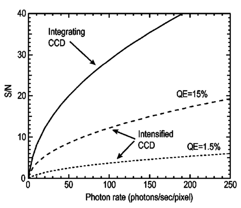
1.

Introduction

The use of light-emitting probes, such as luciferase or fluorescent proteins, as a reporter of gene expression in living cells is a well-established technique for the study of biological activity.¹ Such probes have been widely used in vitro where light detection is easily accomplished using standard photomultiplier tubes or inexpensive charge coupled device (CCD) arrays for imaging applications. Detection of light-emitting probes in vivo within small living animals is also possible due to the semitransparent nature of mammalian tissue,^{2 3 4 5} but improved instrumentation is required, consisting of high-sensitivity low-noise detectors, a more advanced imaging system, and sophisticated software tools for interpreting images.

The ability to track light-emitting cells in small laboratory animals such as mice or rats opens up a wide range of applications in pharmaceutical and toxicological research. These include in vivo monitoring of infectious diseases, tumor growth and metastases, transgene expression, compound toxicity, and viral infection or delivery systems for gene therapy. The ability to detect signals in real time in living animals means that the progression of a disease or biological process can be studied throughout an experiment with the same set of animals without the traditional need to sacrifice for each data point. This results in higher quality data using fewer animals and ultimately will speed the process of screening compounds leading to more rapid drug discovery.

Compared with more traditional structural imaging modalities such as magnetic resonance imaging (MRI) or computed tomography (CT), in vivo bioluminescent imaging offers several advantages. From a practical standpoint, bioluminescent/fluorescent imaging systems are lower cost, have shorter imaging times of <5 min, are easier to use by the nonspecialist, and can image multiple animals at once. In terms of quantitation, MRI/CT systems provide structural size information only, whereas bioluminescent signals provide information about both the location and number of metabolically active cells. Detection of infections in soft tissue such as bacterial pneumonia is also easily accomplished with bioluminescence and is not possible with MRI/CT. Finally, bioluminescent or fluorescent reporters linked to tissue-specific gene promoters provide functional and spatial information on gene expression, opening up an exciting area of research using light-producing transgenic animals.

In this paper, we examine the photonic issues associated with in vivo imaging and describe the design of instrumentation that has been optimized for this application. More specifically, we discuss briefly the tagging of cells with light-emitting markers and look at the trade-offs between bioluminescent and fluorescent probes. The basic physics issues associated with the diffusion of light through tissue are reviewed, along with the spectral properties of tissue. Design of in vivo imaging instrumentation and selection of a CCD is presented, using the general purpose in vivo imaging system (IVIS™) developed at Xenogen as an example. Finally, calibration and signal-to-noise issues are addressed, illustrated using several examples of in vivo images of mice. Most of the photon diffusion and instrumentation design issues discussed in this paper are common to both bioluminescence and fluorescence applications; however, the majority of calculations and image examples in the later part of this paper are for bioluminescent tags (luciferase) because that has been the focus of most of our work to date at Xenogen.

2.

Light-Emitting Reporters

For most in vivo imaging applications, it is desirable to use genetic light-emitting reporters that propagate with the labeled cells as they multiply in an animal. This avoids problems with signal dilution that would be associated with cell division when using exogenous dyes, for example. Luciferases and fluorescent proteins are two common genetic markers. The luciferase enzyme, when combined with the substrate luciferin, oxygen, and ATP, generates light through a chemical reaction resulting in bioluminescence.^{1 6} In the case of fluorescent proteins, the tagged cells must be illuminated with an excitation source in order to fluoresce.

Bioluminescence in mammalian (eukaryotic) cells is accomplished by incorporating the luc gene into the cell’s DNA in order to express the luciferase enzyme. A required substrate, luciferin, is added exogenously and distributes quickly (within minutes) throughout the entire animal. The luc gene originates from the North American firefly, Photinus pyralis, and produces light at an emission peak at ∼560 nm. In prokaryotic cells, the luciferase lux gene from soil bacterium (Photorhabdus luminescens) along with substrate-encoding genes are incorporated into the targeted cell so that both luciferase and luciferin are produced endogenously. The spectra for both types of luciferase are shown in Figure 1. The firefly luciferase is especially attractive for in vivo imaging because the spectrum is very broad and contains a large component above 600 nm where transmission through tissue is higher (see Sec. 3).

Figure 1

Spectral emission measurements for bacterial luciferase in Psuedomonas aeruginosa and firefly luciferase in PC-3M-luc protstate tumor cells. The bacteria is measured on agar while the PC3M cells are measured in a phosphate buffered solution.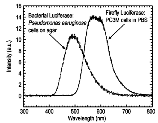

Two common fluorescent proteins are green fluorescent protein and red fluorescent protein or DsRed. The excitation and emission spectra for each are shown in Figure 2. Again, the DsRed is more attractive for in vivo applications because there is significant emission above 600 nm. Note, however, that the excitation remains in the 500–575 nm range where tissue absorption is very high.

Figure 2

Excitation (solid) and emission (dashed) spectra for fluorescent proteins GFP and DsRed (Clonetech Living Colors™ fluorescent proteins).

Bioluminescence has an advantage over fluorescence as an in vivo reporter in that no external light source is required for excitation. This means that background levels are very low compared to those of fluorescent proteins where significant autofluorescence of the tissue surface results from the use of high power external excitation light sources, especially in cases where the luminescent cells are deep in the tissue. Another advantage of bioluminescence is that signals are more easily quantitated because, for tagged cells at a fixed location, the signal level observed on the surface of the animal is directly proportional to the number of cells. In the case of fluorescence, the signal level is related to both the number of cells and the intensity of excitation light, which is difficult to quantify because the excitation light is strongly absorbed as it passes into tissue. In most cases, fluorescent proteins require excitation in the green part of the spectrum where tissue absorption is particularly high. Despite these complications, researchers have made progress in developing diffuse optical tomography codes that treat the propagation of both the excitation and emission through tissue.⁷

For in vitro applications, where cells are not embedded in tissue, fluorescent proteins have an advantage since they are usually brighter than bioluminescent reporters provided that the excitation source is bright enough. It is generally easier to observe individual cells in vitro using fluorescence compared with bioluminescence.

3.

Photon Diffusion in Tissue

Mammalian tissue is a turbid medium that both scatters and absorbs photons.⁸ Photons are scattered due to changes in refractive index at cell membranes and internal organelles. Absorption varies greatly with the type of cell or tissue, but is generally affected by the presence of hemoglobin, which absorbs strongly in the blue-green region of the visible spectrum, but is fairly transparent in the red at wavelengths >600 nm. Typically, for λ>600 nm, the 1/e absorption length is ∼2 cm, while the effective length for scattering is much shorter at ∼0.05 cm (see Refs. 8 and 9 for a review of the optical properties of tissue). In this regime, where scattering is dominant, a significant amount of bioluminescent emission can escape the tissue, but the emission is highly diffuse as illustrated schematically in Figure 3.

Figure 3

In vivo imaging systems view diffuse (scattered) light emitted from an embedded source. The imaging system focuses on the surface of the animal.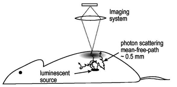

In order to predict in vivo imaging signal levels and spatial resolution as a function of depth, and to help define the requirements for imaging instrumentation, it is important to have a quantitative model for the diffusion of photons in tissue. For the case of homogeneous tissue where the scattering length is short compared with the absorption length (generally true in tissue for λ>600 nm ), photon propagation is well described by a diffusion model.¹⁰ In this model, for continuous waves, the photon fluence ϕ (W/cm²) decays exponentially away from a point source according to

Consider the case of an imaging system viewing down on a homogeneous slab of turbid media with an embedded source as shown in Figure 4. The radiance observed at the tissue surface can be calculated from Eqs. (1) and (2) above with appropriate boundary conditions. Here we use the extrapolated boundary condition,¹¹ which is fairly simple and has been shown to agree well with Monte Carlo simulations and measurements. In this case, an image source is reflected about a plane located a distance z_b above the surface as shown in Figure 4, where

Figure 4

Geometry for the extrapolated boundary photon diffusion model. The extrapolated boundary is a distance z_b above the actual tissue surface.

Figure 5

Surface radiance profile calculated from extrapolated boundary diffusion model (line) and from Monte Carlo simulations (plus symbol). Parameters for this simulation are d=4 mm, μ_a=0.5 cm ⁻¹ , μ_s ^′=15 cm ⁻¹ .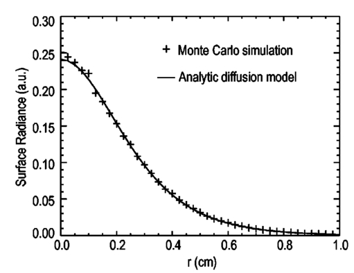

A real animal is neither homogeneous nor a slab shape, but, nevertheless, for source depths that are small compared to the radius of the animal, the above diffusion model can be used to get reasonably good qualitative estimates of signal level and spot size as a function of source depth. In Figure 6(a) the peak radiance (ρ=0) obtained from Eq. (6) is plotted as a function of source depth for three sets of tissue parameters, corresponding roughly to green (550 nm), orange (590 nm), and red (650 nm) wavelengths. At a 1 cm depth the peak signal is attenuated by ∼10⁻² for wavelengths at ∼650 nm while the attenuation is very large ∼10⁻¹⁰ for shorter wavelengths (∼550 nm). Clearly, to observe signals from deep inside the tissue, it is essential to have high sensitivity in the red and near-infrared part of the spectrum. The spot size, or full width at half maximum, of the surface radiance profile is plotted in Figure 6(b). Although wavelengths >600 nm provide much higher signal levels, the trade-off is that the spot size is larger and hence spatial resolution is worse. We note that spatial resolution can actually be much better than the surface spot size indicated in Figure 6(b) if we use the diffusion model with an appropriate fitting algorithm to reconstruct the location and size of the original internal light source.

Figure 6

Calculation of peak intensity (a) and full width at half maximum (FWHM) (b) as a function of source depth for three sets of tissue parameters corresponding roughly to 650 nm (solid), 590 nm (short dash), and 550 nm (long dash). The intensity curves are normalized to one at 1 mm depth.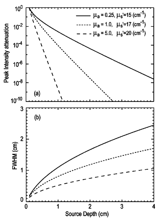

The fact that the absorption coefficient μ_a varies with wavelength results in a redshifting of the peak of the luciferase emission spectrum in vivo compared with in vitro. In Figure 7 we compare the yellow-green firefly (Photinus pyralis) luciferase spectrum measured in vitro in PBS with a subcutaneous tumor in vivo in a nude mouse. The host cell is the PC-3M-luc prostate tumor cell line. The strong attenuation of the signal at wavelengths<600 nm is apparent and is characteristic of the hemoglobin absorption spectrum. In Figure 7, the tumor is only ∼0.5–1 mm deep so some of the emission below 600 nm is still present; however, for sources deeper in tissue, located in internal organs such as the liver, kidney, and lungs, the emission below 600 nm would be completely extinguished.

Figure 7

In vitro (dashed) and in vivo (solid) spectral measurements for firefly luciferase in PC-3M-luc protstate tumor cells. In vivo measurements are for a subcutaneous thigh tumor in a nude mouse.

4.

CCD Selection

Selection of the proper CCD camera is critical for in vivo imaging applications. As seen in Figures 6 and 7, the CCD camera must have high sensitivity or quantum efficiency at wavelengths >600 nm and must have the lowest noise possible in order to detect sources up to a few centimeters deep. An image intensified photon counting CCD camera is one popular choice for many bioluminescent applications. The high-gain image intensifier allows individual photons to be counted with very little noise. However, these cameras, frequently equipped with bialkali photocathodes, suffer from relatively low quantum efficiency (QE) of just 10–15 at 450 nm, dropping to less than 1 at 650 nm as shown in Figure 8 (Hamamatsu C2400-30 Series). Multialkali (S20) and GaAs photocathodes are available that have higher QE above 600 nm, but these tend to have higher thermal noise and cooling issues and are not readily available with large detector areas. Photon counting electronics associated with image intensified systems typically have an electronic threshold that eliminates subthreshold signals and reduces noise. It has been our observation that this threshold can effectively reduce the QE further. Another practical difficulty with photon counting systems is that the count rate is limited by pulse width and counting electronics considerations resulting in limited dynamic range for bright signals. In this case, image brightness must be controlled through some external means such as apertures or neutral density filters.

Figure 8

Quantum efficiency for a bialkali photocathode (triangle), back illuminated (diamond), and front illuminated (square) integrating CCDs.

A better CCD choice for in vivo applications is a cooled back-thinned (and back-illuminated) integrating CCD (e.g., Spectral Instruments 620 Series or Roper Scientific EEV 36-40b). These devices have very high quantum efficiency approaching 85 as shown in Figure 8, and the QE remains high in the red and near-IR spectral regions. Dark current can be a source of noise with integrating CCDs, but cooling the CCD to −105 °C reduces the dark current to near negligible levels, typically<4×10⁻⁴ e/s/pixel for 24 μm pixels. Until recently, cooling detectors to −105 °C required liquid nitrogen, but convenient cryogenic refrigerators have become available making operation at these temperatures relatively easy. There is also electronic noise associated with the CCD readout (read noise) of ∼5 e rms that represents the minimum noise floor that the signal must exceed. Higher spatial resolution is another advantage of integrating CCDs. The Xenogen IVIS™ system typically uses a 25 mm CCD size with a 1024×1024 format and 24 μm pixels (formats 1300×1340 with 20 μm pixels and 2048×2048 with 13.5 μm pixels are also available).

Quantitative comparisons of image intensified versus integrating CCDs can be made by calculating the signal required to achieve a given signal-to-noise ratio for each device. The total noise for a given signal is the rms sum of the read noise, R_N, the noise associated with dark charge, D_c, and the statistical noise associated with the signal itself.¹³ The signal and dark charge follow a Poisson distribution so the noise is simply the square root of the signal. The signal to noise can then be written as (all quantities are in units of electrons)

The signal in Eq. (7) can be increased relative to the read noise by binning pixels together prior to readout. A binning value of 5, for example, means that a 5×5 group of pixels is summed together to form one larger superpixel. In this case, the superpixel has an area of 25 times the original pixel and hence 25 times the signal (and dark current). The read noise remains roughly constant as binning is increased, so binning effectively increases the ratio of signal to read noise. This trade-off of spatial resolution for sensitivity is usually beneficial for in vivo imaging where signal levels are low and the diffuse images do not demand high spatial resolution.

A comparison of S/N from Eq. (7) for integrating and intensified CCDs is shown in Figure 9. For this figure we assume the high resolution CCD described above is binned to ∼200×200 pixels, i.e., bin=5. For integrating CCDs we have R_N∼5 electrons, D_c∼0.01τ electrons/pixel, and Q_E∼0.85. Photon counting CCDs do not have a dark current specification, but for a typical 26 mm bialkali photocathode there is a thermal emission of ∼10 electrons/s/image which gives an effective dark current of 2.5×10⁻⁴τ electrons/pixel. The read noise is assumed to be zero for the photon counting CCD and quantum efficiencies of 15 (∼450 nm) and 1.5 (∼600 nm) are plotted in Figure 9 for this device. For very low signals (S/N∼1), both the integrating and intensified (QE=15) CCDs give similar performance. However, at S/N∼10, the intensified CCD requires about five times as much signal as the integrating CCD. Physically, what is happening here is that for S/N∼1 the higher QE of the integrating system combined with higher read noise ends up giving essentially the same S/N for the same signal as the intensified CCD. But as the S/N increases to 10, the read noise and dark charge noise become negligible compared with the signal noise itself, and so the higher QE of the integrating system ends up giving better performance. As seen in Figure 9, at the red wavelengths of interest for in vivo imaging, the low QE gives very poor performance.

Figure 9

Comparison of S/N for an integrating CCD (solid) and an intensified CCD (dashed). Two quantum efficiencies are plotted for the intensified CCD corresponding to λ=450 nm (QE=15) and λ=600 nm (QE=1.5).

5.

Imaging System Design

In consideration of the above arguments, a general purpose in vivo imaging system (IVIS™) has been developed at Xenogen based on a cooled back-illuminated integrating CCD. A schematic of the instrument is shown in Figure 10. The CCD camera is located on top of a light-tight imaging chamber. The door to the chamber is made extremely light tight through the use of a double baffle seal while the remainder of the enclosure is constructed in such a way as to minimize any penetrations into the box. Light is collected from the specimen and imaged onto the CCD using a fast 50 mm f/1 lens. The sample stage moves up and down to vary the field of view (FOV) from 10–25 cm. A seven-position filter wheel is also provided to enable spectral imaging capability. The sample stage, lens focus, f/stop, and filter wheel are all stepper motor controlled through Xenogen’s Living Image^® control software. Light-emitting diodes (LEDs) are located on the top plate to illuminate the specimen for photographic images. Other convenient features include a gas anesthesia system and a heated sample shelf to help maintain an animal’s body temperature during anesthesia.

Figure 10

Illustration of the IVIS™ imaging system.

A typical in vivo image is shown in Figure 11 where 10⁶ cells tagged with bacterial luciferase (Strep. pneumonia) were administered through the trachea with a ball-tipped needle. The sequence of steps required to produce this image can be summarized as follows. For the initial image (start of an experiment) bioluminescent cells are injected into the animal. If using firefly luciferase, then the luciferin substrate must also be injected prior to each image, while for bacterial luciferase the substrate is produced endogenously. The animal is then anesthetized with isoflurane and placed in the imaging chamber. A gas manifold with a nose cone is provided in the chamber to maintain anesthesia during imaging (see top of Figure 11). In a typical image sequence, the LEDs are turned on and a photographic image is acquired and displayed with a grayscale color table, equivalent to black and white photograph. Then the LEDs are turned off and a longer exposure image of the bioluminescent (or fluorescent) light is taken. The bioluminescent image is overlaid on top of the photographic image using a pseudo-color intensity scale as seen in Figure 11, where red indicates the highest intensity and violet the lowest intensity. The exposure time and f stop were 0.2 s, f/8 for the photographic image and 30 s, f/1 for the bioluminescent image. Note that the individual lobes of the lungs can be distinguished in this image.

Figure 11

Pneumonia model in a Balb/c mouse with 10⁶ cells of Strep. pneumoniae-xen10 administered through the trachea. Image taken at 42 h with a 30 s integration time and binning=10. The pseudocolor bioluminescent image is overlaid on top of a grayscale photographic image of the mouse. Color bar units are in digitizer units, or ADU.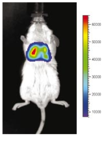

The units on the color bar in Figure 11 and all other images shown in this paper are analog-to-digital converter units, or ADU. The signal in ADU is related to the number of photoelectrons in a pixel by S _ADU =S_eG where G is the CCD amplifier gain. Typically, for the CCD cameras used in this study, G∼1 so it is appropriate to equate S _ADU ∼S_e.

6.

Calibration and Signal-to-Noise Estimates

Absolute intensity calibration of the CCD camera and overall imaging system is necessary to calculate brightness (in physical units) of luminescent cells and to estimate the number of cells inside an animal from the intensity of the surface image. To accomplish this, we utilize an absolutely calibrated 8 in. integrating sphere from Optronic Laboratories, Inc. (OL Series 425 Variable Low-Light-Level Calibration Standard). The integrating sphere is illuminated with a tungsten lamp, and the light level entering the sphere can be controlled using a set of reducing apertures and by moving the lamp away from the aperture. This combination allows very low radiance levels of ∼10⁻¹⁰ W/cm ²/sr (sr=steradian) across the 2 in. output aperture of the sphere. By imaging this aperture, counts detected by the CCD camera digitizer (ADU) can be converted to physical units of radiance in W/cm²/sr or photons/s/cm²/sr. The camera calibration depends on f-stop and shelf position. A typical calibration for a wide open lens (f/1) and a 15 cm FOV is 4×10⁵ photons/s/sr/cm ² at the object plane per ADU/s/pixel at the CCD (for 24 μm pixel size and λ=600 nm. ) To give an example of sensitivity, if we assume a 5 min image with binning of 8 (64 pixels grouped together to form a larger pixel) and a total noise of 7 ADU per binned pixel, then the minimum detectable radiance is

An in vitro image of a 96-well plate containing a dilution series of bioluminescent bacteria (Pseudomonas aeruginosa) is shown in Figure 12. The cell count per well ranges from 5000 down to 150. The 150-count well is barely visible above the CCD noise and represents the minimum detectable number of cells for this particular cell line in a 96-well plate. There are about 60 binned (bin=10) pixels in a well giving ∼2.5 cells per pixel sensitivity in this case, consistent with the discussion above.

Figure 12

Image of well plate containing Pseudomonas aeruginosa cells tagged with bacterial luciferase (top). Cell counts range from 5000 on the left to 150 on the right. The lower plot shows the total counts per well versus the number of cells, indicating good linearity.

Of particular interest to the application of in vivo imaging is the minimum observable cell as a function of depth in an animal. The number of CCD signal electrons, S_e, required to give a certain signal-to-noise ratio, S_N, is given by Eq. (8). We can combine this with Eq. (6) to find the minimum number of cells that can be detected at a depth d. Defining a normalized radiance as L_n≡L_z=0/P and replacing the emission power P with the integrated photon count, which is given by C_nρ_cτ where C_n is the number of bioluminescent cells, ρ_c is the photon emission rate per cell, and τ is the integration time, we can write

Figure 13

Cell count vs source depth calculated using the diffusion model for three different S/N ratios. Solid lines are μ_a=0.25 cm ⁻¹ (λ>600 nm) and dashed lines are μ_a=1.0 cm ⁻¹ (λ<600 nm). A scattering coefficient of μ_s ^′=15 cm ⁻¹ and a bioluminescent emission of 30 photons/cell/s was used for all curves.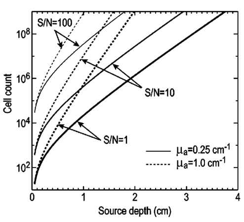

The results from Figure 13 are in good agreement with measurements in real animals. In Figure 14(a) we show images of PC3M-luc prostate tumor cells injected subcutaneously into a nude mouse. Cell counts of 500, 1000, 10⁴, and 10⁵ were injected into the thigh of each animal. In this case, 500 cells is close to the minimum cell count that can be observed. The sum of the counts in an Region of Interest (ROI) surrounding each spot is plotted in Figure 14(b). For comparison, in vitro measurements of the same cell counts are also shown in Figure 14(b). A deep-source lung signal is shown in Figure 15. For this animal, 4×10⁶ PC3M-luc cells were injected into a tail vein, where cells are promptly transported to the lungs. The peak signal levels and signal-to-noise values from both Figures 14 and 15 are given in Table 1. The signal units in this table are ADU, but since the CCD amplifier gain is ∼1 we can assume S _ADU ∼S_e for comparison with Figure 13. Although the data in Table 1 are limited, the S/N versus depth trend is in qualitative agreement with that predicted in Figure 13.

Figure 14

(a) Subcutaneous injection of PC3M-luc prostate tumors cells. Cell counts from left to right are 10⁵, 10⁴, 1000, and 500. (b) Sum of counts from ROIs around each site in (a), normalized to a 1 minute image time (red). Counts for cells in a 96-well plate are also shown (blue). There are two images and hence two data points for each cell count number.

Figure 15

Image showing bioluminescence from the lungs after an intravenous tail injection of 4×10⁶ PC3M-luc cells. Imaging time is 1 min and binning=8.

Table 1

The signal-to-noise calculations above only consider the CCD and intrinsic signal noise. In addition, there can be other sources of background light that create what is effectively a higher noise floor. As seen in Figure 14(a), background light can be observed on the animal with the 500-cell injection. This background level is small and is usually only a factor when looking for the very lowest bioluminescent signals. The background emission can result from phosphorescence of the skin, fur, or impurities on the animal. There also appears to be a low-level light emission due to metabolic activity in live animals, although this is not very well understood at the present time. Regardless of the source, every effort must be made to reduce the background light in order to approach the intrinsic noise floor of the CCD camera.

As a final example of the power of in vivo imaging, we show an example of tumor metastases in Figure 16. Here 5×10⁶ breast cancer cells (MDA-MB-231-luc) were injected into a tail vein and this image was taken at week 14 after injection. The image shows clear metastatic signals from the lungs and lower body organs. These tumors are small and certainly would not have been palpable externally. The animal was dissected shortly after this image was taken, and ex vivo signals were found in the lungs, spine, adrenal glands, and lymph nodes.

Figure 16

Dorsal (left) and ventral (right) views of metastatic signals from breast cancer cell line MDA-MB-231-luc, week 14 after intravenous injection of tumor cells. Imaging time is 2 min and binning=4.

7.

Conclusion

In vivo imaging of cells or viruses tagged with light-emitting probes promises to be an important technology for the study of biological activity, the screening of potential drugs, and the assessment of toxicological effects of compounds. Both bioluminescent luciferase and fluorescent proteins are potential tags that can be used, although bioluminescence has a significant advantage due to extremely low backgrounds. Long-wavelength (>600 nm) probes will give the best signal levels in mammalian tissue due to lower absorption in tissue. The use of state-of-the-art cooled integrating CCD cameras along with imaging chambers optimized for in vivo applications allow the detection of bioluminescent signals throughout the body of small laboratory animals such as mice or rats. Experiments with luciferase tagged cells have demonstrated that minimum cell counts in the range of ∼500 cells can be detected subcutaneously, while higher cell counts are required for larger depths in tissue. The sensitivity of detection is adequate to observe metastases of cancer cells, demonstrating the potential of in vivo imaging technology.