1.

Introduction

Fluorescence spectroscopy is a nondestructive optical method extensively used to probe complex biological systems, including cells and tissues for biochemical, functional, and morphological changes associated with pathological conditions. Such an approach has potential for noninvasive diagnosis in vivo.^{1 2 3} Fluorescence measurements can be categorized as either static (steady state or time integrated) or dynamic (time- resolved). While steady state techniques provide an integrate spectrum over time that gives information about fluorescence emission intensity and spectral distribution, time-resolved techniques measure the dynamically evolving fluorescence emission, providing additional insight into the molecular species of the sample (e.g., the number of fluorescence species and their contribution to the overall emission) and/or changes in the local environment.^{2 3}

Two methods for time-resolved fluorescence measurements are widely used: The time-domain and the frequency-domain techniques. For the time-domain method, the sample is excited with a short pulse of light (typically nanosecond or shorter), and the emission intensity is measured following excitation with a fast photodetector. In the frequency domain, an intensity-modulated light induces the sample fluorescence. Due to the fluorescence relaxation lifetime of the sample, the emitted wave is delayed in time relative to the excitation, inducing a phase-shift, which is used to calculate the decay time.³ The analytical approaches described here are applicable for analysis of time-domain data. The frequency-domain analysis is not discussed in this paper.

Analysis of time-resolved data from fluorescent systems includes determination of the intrinsic fluorescence intensity decay (fluorescence impulse response function, IRF), identification of a set of fitting parameters that best describe the characteristics of the fluorescence decay, and characterization and discrimination/classification of the fluorescent system based on those parameters.²

In the context of time-domain measurements, the fluorescence IRF contains all the temporal information of a single fluorescence decay measurement. The IRF is the system response to an ideal δ function excitation. In practice, the excitation light pulses are, typically, at least several picoseconds wide. Thus, they should be taken as a train of δ functions with different amplitudes; each one initiating an IRF from the sample, with an intensity proportional to the height of the δ function. The measured intensity decay function is the sum of all IRFs starting with different amplitudes and at different times. Mathematically, the measured fluorescence intensity decay data is given by the convolution of the IRF with the excitation light pulse. Thus, to estimate the fluorescence IRF of a compound, the excitation light pulse must be deconvolved from the measured fluorescence intensity pulse.³

When the excitation light pulse is sufficiently short, resembling a δ function excitation, the measured fluorescence decay would closely resemble the intrinsic IRF.⁴ Although very short excitation light pulses can currently be generated using femtosecond lasers, due to their lack of general availability picosecond light sources are still the most commonly used for time-resolved measurements.³ Therefore, in many cases the intrinsic fluorescence IRF of the investigated compounds will have lifetimes on the order of the excitation light pulse width, and subsequently, an accurate deconvolution technique becomes crucial.

Deconvolution methods are usually divided into two groups⁵: those requiring an assumption of the functional form of the IRF, such as the nonlinear least-square iterative reconvolution method^{6 7} and those that directly give the IRF without any assumption, such as the Fourier⁸ and Laplace transform methods,⁹ the exponential series method,⁵ and the stretched exponential method,¹⁰ among others. In addition, an alternative approach known as global analysis, in which simultaneous analysis of multiple fluorescence decay experiments are performed, has proven useful for both time- and frequency-domain data.¹¹ Among these methods, however, the most commonly used deconvolution technique is the nonlinear least-squares iterative reconvolution (LSIR) method.^{5 6 7} This technique applies a least-squares minimization algorithm to compute the coefficients of a multiexponential expansion of the fluorescence decay. In complex biological systems, fluorescence emission typically originates from several endogenous fluorophores and is affected by light absorption and scattering. From such a complex medium, however, it is not entirely adequate to analyze the time-resolved fluorescence decay transient in terms of a multiexponential decay, since the parameters of a multiexponential fit cannot readily be interpreted in terms of fluorophore content.^{3 10} Moreover, different multiexponential expressions can reproduce experimental fluorescence decay data equally well, suggesting that for complex fluorescent systems there is an advantage in avoiding any a priori assumption about the functional form of the IRF decay physics.

Expansion on the discrete time Laguerre basis as means of deconvolving the intrinsic properties of a dynamic system from experimental input-output data was initially proposed by Marmarelis¹² and was applied to linear and nonlinear modeling of different physiological systems including renal autoregulation and autonomic control of heart rate.^{13 14} A Laguerre based deconvolution technique was recently reported as a variant of the LSIR technique, in which the fluorescence IRF is expressed as an expansion on the discrete time Laguerre basis instead of a weighted sum of exponential functions.¹⁵ The Laguerre deconvolution technique has been previously applied to optical spectroscopy of tissues with promising results to the analysis of time-resolved fluorescence emission data from artherosclerotic lesions,^{1 2} and temporal spread functions of transmitted ultrafast laser pulses through different types of human breast tissue.¹⁶ However, a formal evaluation of this technique, as it applies to fluorescence measurements, has not been reported. In this paper, the performance of the Laguerre deconvolution technique is analyzed in terms of accuracy and speed for retrieving the fluorescence IRF and compared to that of the multiexponential LSIR deconvolution technique.

Although the main objective of a deconvolution technique is to retrieve accurately the intrinsic fluorescence intensity decay characteristics of a compound, it is also very important that such a technique provides a unique representation of the intrinsic temporal fluorescence dynamics that allow further characterization of the investigated biological system. The study of Zacharakis et al.;¹⁶ on the analysis of the temporal spread of transmitted ultrafast laser pulses through tissue represents the only attempt to directly use the Laguerre expansion coefficients to characterize biological systems, yielding promising but very preliminary results.¹⁶ Although the Laguerre deconvolution technique was used for the analysis of time-resolved fluorescence data from fluorescent constituents in tissues as well as tissue samples,^{1 2 15} the potential of Laguerre expansion coefficients for direct characterization and discrimination of fluorescence from biological systems has not been reported. Because these coefficients inherently contain information about the amplitude (intensity) and the relaxation time of a dynamic system, this paper investigates properties of Laguerre expansion coefficients that allow direct characterization of fluorescent system.

In summary, the goals of this paper were (1) to assess the performance of the Laguerre deconvolution technique in terms of its accuracy and speed for retrieving the intrinsic fluorescence decay from simulated and lifetime fluorescence standards data; (2) to investigate the analytical properties of the Laguerre expansion coefficients and to demonstrate their potential to directly characterize biochemical systems in terms of their fluorescence intensity decays; (3) to determine the potential use of Laguerre coefficients for quantitative interpretation of fluorescence data; and (4) to introduce a new method for prediction of concentration of mixtures of biochemical components that take advantage of the Laguerre coefficients information content.

2.

Theoretical Approach

3.

Generation of Time-Resolved Fluorescence Data

4.

Technique Evaluation and Validation

4.1.

Simulated Data

A simulated time-resolved fluorescence intensity decay (τ=4.1 ns at a medium noise level), its corresponding estimation by the Laguerre deconvolution method (L=5) , and the laser pulse (solid black) are shown in Fig. 1. The residuals are <2 of the peak fluorescence amplitude and they appear randomly distributed around zero. The autocorrelation function of the residuals does not contain low-frequency oscillations characteristic of nonrandom residuals, and is mostly contained within the 95 confidence interval centered around zero. These observations indicate an excellent fit between the synthetic and estimated fluorescence decays, showing that the fluorescence IRF was properly estimated with the deconvolution algorithm based on the Laguerre expansion technique. The results for the same sample fluorescence decay using the multiexponential approach (P=3), presented in Fig. 1, showed similar results. One important detail depicted in Fig. 1 is that the residuals and autocorrelation functions corresponding to both the Laguerre and multiexponential fits look very much alike. This is explained by the fact that both techniques were able to accurately fit the true synthetic time-resolved decay data, leaving out just the additive white noise component of the artificial data.

Figure 1

Laguerre and multiexponential deconvolution of the excitation laser pulse (solid black) from a simulated fluorescence decay (solid gray, τ=4.1 ns) . The extimated fluoresccence decays (dotted black) overlap the simulated fluorescence decay. The residuals and their autocorrelation function indicate excellent fit between the synthetic and the estimated fluorescence decays.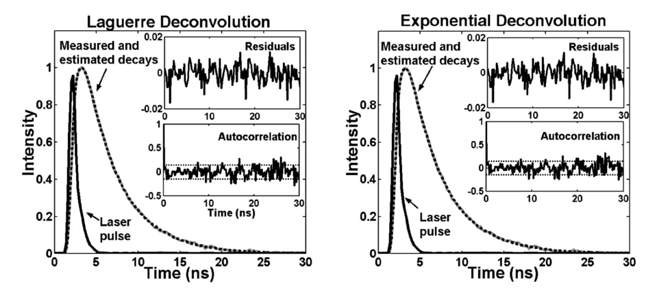

The performance of Laguerre and multiexponential deconvolution techniques along the lifetime range of 0.3 to 12 ns was assessed by means of the relative error between the real and the estimated lifetime (RLE) values, and the normalized mean square error (NMSE). Similar performances were obtained for both techniques: the RLE values were found below 1, 2, and 4, whereas the NMSE values were smaller than 0.04, 0.3, and 0.9 for the low-, medium-, and high-noise-level groups, respectively.

To investigate the effect of the number of LF (chosen to expand the fluorescence IRF) on the estimation of the intrinsic fluorescence decay, the synthetic data was deconvolved using Laguerre expansions of different orders (three to six LFs). For decays with lifetimes ranging from 1 to 8 ns, the IRF expansion with five LF yielded the best estimation of the fluorescence emission decay (RLE<2). The best estimate for fast decays (τ_f<1 ns) and for slow decays (τ_f>8 ns) were obtained using an expansion of six LFs and three to four LFs, respectively. For the multiexponential deconvolution method, a good estimation of the IRF (RLE<2) was yielded by biexponential expansion for slow decays and triexponential expansion for fast decays.

As stated, it is important that a deconvolution technique provides a representation of the intrinsic temporal fluorescence dynamics to be used for further characterization of the investigated compound. Both the multiexponential and Laguerre deconvolution techniques summarize the temporal fluorescence intensity decay information in terms of the parameters of the model they use to represent the fluorescence IRF: (1) the preexponential factors (a_i) and the decay constants (τ_i) for the case of the multiexponential approach and (2) the Laguerre α parameter and the c_j expansion coefficients for the case of Laguerre approach. Therefore, a natural attempt to characterize a compound in terms of its fluorescence lifetime information is to utilize either the multiexponential or the Laguerre model parameters.

To investigate whether these model parameters reflect by themselves the fluorescence temporal information of the investigated compound, the correlation coefficients between the actual lifetime values of the simulated data and the model parameters (first two exponential parameters and first three Laguerre expansion coefficients) were computed. For a bivariate case, the correlation coefficient (−1<r<1) is defined as the covariance between the two variables normalized by the variances of each variable, and measures the strength of the linear relationship between the two variables. A correlation coefficient r=−1 indicates a perfect negative (inverse) linear dependence, r=0 indicates no linear dependence, and r=1 indicates a perfect positive linear dependence.⁴

The first three Laguerre expansion coefficients as a function of the radiative lifetime between 4 and 5 ns and the correlation coefficients are shown in Fig. 2. We can clearly observe the first and third expansion coefficients were positively correlated with the intrinsic decay lifetime, whereas the second expansion coefficient was negatively correlated with the intrinsic lifetimes. All three Laguerre expansion coefficients (LEC-1 to LEC-3) were highly correlated to the real lifetime values (r>0.95). This result indicates that each of the Laguerre expansion coefficients capture and reflect the temporal relaxation of the IRF, and thus can be further used for the characterization of the investigated compound.

Figure 2

Correlation between the actual lifetime values of the simulated data with the Laguerre expansion coefficients (LEC-1 to LEC-3, left panels) and the multiexponential LSIR parameters (right panels).

Plots of the biexponential fast (τ₁) and slow (τ₂) decay constants and of the relative contribution of the fast exponential [a₁/(a₁+a₂)] as a function of the radiative lifetime between 4 and 5 ns are also shown in Fig. 2. For this particular lifetime range, only one of the time-decay constants, the slow decay constant (τ₂), was positively correlated (r=0.82±0.01) with the lifetime values. The remaining time decay constant and the normalized preexponential factors were not correlated with the lifetime values (r=0.55±0.02 and r=0.54±0.03, respectively).

4.2.

Experimental Data

To investigate the accuracy of the Laguerre deconvolution method for retrieving fluorescence decays from experimental data, a number of lifetime fluorescence standards with a broad range of relaxation lifetimes were measured in solutions. The lifetimes retrieved using both the Laguerre and the multiexponential deconvolution methods were compared with values from the literature.³ The results of this analysis are presented in Table 1 [mean±standard error (SE)]. Short-lived fluorophores, such as rose bengal, with lifetimes ranging in the hundreds of picoseconds could be reliably retrieved by the Laguerre deconvolution technique. This is shown in Fig. 3 for a fluorescence intensity decay measurement from RB in methanol at 580 nm. The fluorophore intensity decay data was best fitted to Laguerre models of L=3 or L=4 and to a single-exponential decay. Both methods yielded very good fits, although in this particular example, the Laguerre approach performed better than the multiexponential method, as indicated by the smaller Laguerre residuals (top insets). Both the Laguerre and the exponential methods yielded similar intrinsic fluorescence decays (IRF) with lifetime values of 0.456±0.004 and 0.4±0.006 ns, respectively, which were in good agreement with previously reported data.³

Figure 3

Laguerre and multiexponential deconvolution of the excitation laser pulse (solid black) from a measured fluorescence decay from RB in methanol at 580 nm (solid gray). The estimated fluorescence decays (dotted black) overlap the measured fluorescence decay. The residuals indicate excellent fit between the measured and the estimated flourescence decays. The estimated IRF using both methods present very similar decay characteristics.

Table 1

Lifetime values (mean±SE) of fluorescence standard dyes estimated using the Laguerre and exponential deconvolution techniques.
Sample	Solvent	Lifetime (ns)			Wavelength (nm)
		Laguerre	Exponential	Literature3
RB	Ethanol	0.769±0.005	0.702±0.004	0.850	590
RB	Methanol	0.457±0.004	0.400±0.006	0.540	580
RdmB	Ethanol	2.872±0.015	2.880±0.006	2.850	590
RdmB	Deionized water	1.533±0.057	1.531±0.024	1.520	580
9/CA	Ethanol	11.746±0.026	11.630±0.020	11.850	445

Similarly, measurements of RdmB in ethanol and methanol demonstrated the ability of the Laguerre method to accurately resolve nanosecond and subnanosecond fluorescence lifetimes (Fig. 4), which is of especial importance since a number of biologically relevant fluorophores such as elastin and collagen are known to emit at these time scales.^{2 15} The RdmB fluorophore intensity decay data was best fitted to Laguerre models of L=4 and to a single exponential decay. Both methods yielded very good fits as it can be seen in Fig. 4.

Figure 4

Laguerre and multiexponential deconvolution of the excitation laser pulse (solid black) from a measured fluorescence decay from RdmB in ethanol at 590 nm (solid gray). The estimated fluorescence decays (dotted black) overlap the measured fluorescence decay. The residuals indicate excellent fit between the measured and the estimated fluorescence decays. The estimated IRF using both methods present very similar decay characterics.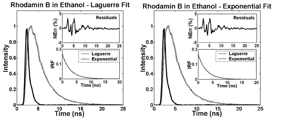

Finally, to assess the ability of the Laguerre technique to retrieve long fluorescence lifetimes, the fluorescence decay of 9-cyanoanthracene (9CA) in ethanol were also deconvolved (Fig. 5). Both the Laguerre and the exponential methods yielded similar intrinsic fluorescence decays with lifetime values (Table 1) also in agreement with previous reports.³ The 9CA fluorophore intensity decay data was best fitted to Laguerre models of L=2 and to a single exponential decay, and very good fits were attained by the two methods as observed in Fig. 5. Similar to the results on the simulation data, it was observed that deconvolution of long-lived fluorophores (e.g., 9CA) require fewer LFs for expansions when compared with the short-lived compounds (e.g., RB and RdmB).

Figure 5

Laguerre and multiexponential deconvolution of the excitation laser pulse (solid black) from a measured fluorescence decay from 9/CA in ethanol at 445 nm (solid gray). The estimated fluorescence decays (dotted black) overlap the measured fluorescence decay. The residuals indicate excellent fit between the measured and the estimated fluorescence decays. The estimated IRF using both methods present very similar decay characteristics.

To compare the computational time of both the Laguerre and the multiexponential deconvolution techniques, 250 sets of 9CA time-resolved fluorescence data at several wavelengths (400 to 650 nm) were deconvolved using both techniques, and the deconvolution time was measured for each set of data. The average computational time was 33.1±0.86 ms for the Laguerre deconvolution with five LFs, and 101.4±1.6 ms for the LSIR deconvolution with a single exponential. Both methods were implemented in Matlab-6.5 (The MathWorks, Natick, MA) and executed on an IBM-compatible workstation (Intel Xeon processor, 2.0 GHz).

5.

Discussion

Although a multiexponential deconvolution has the potential to accurately retrieve the fluorescence IRF of complex biomolecular systems, the parameters of a multiexponential fit cannot readily be interpreted in terms of number of fluorophore content.^{3 5} Changes of a fluorophore environment, proteins conformations or cross-links, also would result in different intensity decay for a single fluorophore,^{3 5} thus it is not practical to consider individual decay times. Moreover, very different multiexponential expressions can reproduce the same experimental fluorescence intensity decay data equally well as demonstrated with the simulation results presented here, in which synthetic decay data generated by a four-exponential model was accurately deconvolved by multiexponential models of different orders from two to four exponential components. This and previous reported evidence^{3 5 10} support the conclusion that for complex fluorescence systems, there is an advantage in avoiding any assumption about the functional form of the fluorescence decay law. Further, this suggests that the Laguerre deconvolution technique is a suitable approach for the analysis of time-domain fluorescence data of complex systems, since this technique has the ability to expand intrinsic fluorescence intensity decays of any form, without any a priori assumption of its functional form.

While the results from both simulation and lifetime fluorescence standard support the conclusion that the Laguerre method performs similarly to the multiexponential method in terms of accuracy for retrieving the fluorescence IRF, one advantage of the Laguerre method is that for any value of the Laguerre parameter α, the corresponding basis of LF is a complete orthonormal basis. Thus, it is certain that an expansion of the fluorescence IRF on the LF basis can always be found, and even more important, the set of expansion coefficients are unique for a defined Laguerre basis. Our results showed that three to six LFs are sufficient to expand fluorescence decays with lifetime values ranging from 0.3 to 12 ns, which are times relevant for the emission of tissue endogenous fluorophores. Generally, an accurate estimation of slow decays requires fewer LFs for expansion (less than three) than for the fast decays (larger than five). In contrast, deconvolution with the multiexponential approach may yield more than one solution, even when the number of exponential or the values of the decay constants are prefixed. The span of possible solutions of a multiexponential expansion can be significantly reduced by fixing a priori the values of the decay constants, as was proposed in the exponential series method proposed by Ware et al.;⁵ Note, however, that deconvolution with the exponential series method is successful only when the prefixed decay constants are commensurate with the investigated fluorescence decay.

Another advantage of the Laguerre deconvolution over the multiexponential LSIR results from the different methods required to estimate the expansion parameters. The Laguerre expansion technique uses a least-squares optimization procedure to determine the coefficients of the Laguerre expansion of the system dynamics.¹² For a defined Laguerre basis, i.e., given values of the parameter α and the number of the LFs, the problem of finding the expansion coefficients is reduced to solving an overdetermined system of linear equations [given in Eq. (5)], which represents a linear least-squares minimization problem. The same property holds even for the estimation of nonlinear dynamics that can also be formulated in terms of linear equations using the Laguerre expansion technique.^{12 13 14} In contrast, traditional multiexponential LSIR techniques require the estimation of intrinsic nonlinear parameters (the decay constants), which represents a nonlinear least squares problem. Although very robust and efficient nonlinear least square algorithms are currently available, such as the Gauss-Newton and Levenberg-Marquardt methods,²² solving a linear least-squares problem (Laguerre technique) is a much simpler and less computationally expensive problem than finding a nonlinear least square solution (through a multiexponential technique). This was clearly supported by the results described here on the speed of computational analysis, showing that the Laguerre deconvolution technique convergences to a correct solution approximately three times faster than the monoexponential deconvolution. The convergence speed would become more significant when a biexponential or higher order multiexponential expansion is used. This specific advantage of the Laguerre method becomes even more important in the context of application of lifetime fluorescence spectroscopy to clinical research of tissue diagnosis, where the speed of data analysis is of crucial importance.

Analysis of correlations coefficients (r) demonstrated that each Laguerre expansion coefficient is highly correlated with the intrinsic lifetime value, suggesting that the use of these coefficients has potential, as a new approach, for the direct characterization of biochemical compounds in terms of their fluorescence emission temporal properties. For the case of the multiexponential deconvolution, although the estimated (computed) average lifetime is always correlated with the intrinsic radiative lifetime, the individual multiexponential parameters (decay constants and preexponential coefficients) may not necessarily be correlated to the intrinsic lifetimes. This was shown in the simulations results, where only one of the decay constants was correlated with the lifetime. This lack of correlation between individual multiexponential parameters and the lifetime occurs because the multiexponential model does not represent an orthogonal expansion of the fluorescence IRF; therefore, the estimated fitting parameters are not independent from each other.^{3 23} This condition implies that the value of one specific parameter is determined not only by the data to be fitted, but also by the value of the other fitting parameters; thus, reducing the correlation between the actual lifetimes and the estimated values of the multiexponential parameters. In contrast, since the Laguerre basis provides an orthogonal expansion of the IRF, the value of each expansion coefficient depends exclusively on the data to be fitted, making them highly correlated to the actual lifetime values.

This paper also demonstrated that the Laguerre expansion coefficients have potential for quantitative interpretation of fluorescence decay. A new method for the prediction of concentrations in a mixture was introduced here and successfully tested on fluorescence standards components (RdmB and RB). Moreover, using only fluorescence decay information from a narrow spectral range, this method yielded improved prediction of the fluorophore concentrations when compared to that obtained using traditional methods of spectral analysis (PCR and PLS). One possible explanation for this result is that spectral methods use the information derived from spectral distribution of fluorescence intensity, while the proposed Laguerre method uses both the amplitude and temporal information of the fluorescence emission from a predefined narrow spectral range. Emission spectra of RdmB and RB are highly overlapped,³ thus spectral emission alone would provide limited information for the prediction of their relative concentration. However, RdmB and RB present different fluorescence decay characteristics, which were taken into account together with the amplitude information when the Laguerre coefficients were applied for concentration prediction. Although in this paper, the proposed Laguerre method analyzes only the amplitude and temporal information of the fluorescence emission from a predefined narrow spectral range, the Laguerre expansion coefficients corresponding to fluorescence IRF taken at multiple emission wavelengths also reflect the spectral information of the fluorescence emission. This spectral information could also be integrated into a more advanced method for characterization and discrimination of a biological system.

It is also noteworthy that an analogous method for the prediction of concentrations in a mixture of biochemical components based on the multiexponential model of intrinsic fluorescence decay could also be implemented. Since such a method would also use both the amplitude and temporal information contained by fluorescence data, it would most likely yield a performance similar to that of the Laguerre method presented in this paper. However, a method based on the multiexponential expansion would require that the decay constants be chosen a priori. Therefore, one disadvantage of this approach would represent the necessity for a good guess of the decay constants (these must be commensurate with the investigated fluorescence decays) to ensure an acceptable prediction of the investigated concentrations.⁵ A further requirement for such a technique would be that the number of exponential terms used should be equal to or greater than the number of biochemical concentrations to be retrieved. Therefore, the larger the number of component assumed to be present in the investigated biological system, the more exponential terms are required, and a large number of decay constants must be guessed, making its application difficult. The Laguerre-model-based method for concentration estimation requires only predefining the Laguerre parameter α, which can be chosen from the observed decay data.¹²

All these findings taken together suggest that the application of the Laguerre expansion method (and specifically, of the expansion coefficients) represent a promising approach for the quantification of relative concentrations of different biochemical compounds in biological systems, and their subsequent characterization and discrimination. Application of the Laguerre deconvolution techniques can result not only in accurate analysis of fluorescent systems without a priori knowledge of underlying fluorescence dynamics but also facilitates reduction of data processing time. This method can be easily adapted for the analysis of time-resolved fluorescence data from tissues, and thus it has potential impact on applications of fluorescence lifetime to in vivo spectroscopic diagnostics of diseased tissues (e.g., arterial plaques and tumors) and functional imaging microscopy of living cells.

In conclusion, this work demonstrated that numerical deconvolution of fluorescence IRF using a nonparametric expansion in a discrete-time Laguerre basis enables accurate estimation of the intrinsic fluorescence intensity decays for a broad range of lifetime values. Although the main objective of a reliable deconvolution technique is to accurately retrieve the intrinsic fluorescence decay of a compound, it would also be very important for such technique to provide a unique representation of the intrinsic fluorescence dynamics that can be used for further characterization of the investigated biological system. Taking into account this consideration, our results demonstrated that the Laguerre deconvolution method includes a number of interesting properties and potential advantages over the classical multiexponential LSIR. These include faster convergence to a correct solution, high correlation between the expansion coefficients and the intrinsic lifetime values, and the potential for directly quantifying the relative concentrations of different biochemical compounds in biological systems. These characteristics suggest that the use of the Laguerre expansion coefficients represents a new reliable and powerful approach for the characterization and discrimination of biological systems, in terms of their fluorescence emission intensity amplitude and temporal or lifetime characteristics. Future work will investigate the application of this approach to analysis of time-resolved fluorescence data obtained from in vivo measurements in diseased tissue including atherosclerotic lesions and brain tumors.