Clustered targets imaged by optical tomography guided by ultrasound

Yan Xu; Chen Xu; Quing Zhu

doi:10.1117/1.3600773

1 July 2011 Clustered targets imaged by optical tomography guided by ultrasound

Yan Xu, Chen Xu, Quing Zhu

Author Affiliations +

Journal of Biomedical Optics, Vol. 16, Issue 7, 076018 (July 2011). https://doi.org/10.1117/1.3600773

Abstract

Clustered small breast lesions may be present in the neighboring areas and are difficult to accurately resolve and quantify in diffuse optical tomography. In addition, larger cancers are often accompanied by clustered satellite lesions in the neighboring areas, which are also difficult to resolve and quantify. To improve the light quantification of clustered lesions, a new multi-zone reconstruction algorithm guided by co-registered ultrasound (US) was investigated using simulations, phantoms, and clinical examples. This method separated one larger region-of-interest (ROI) into several ROIs based on the location information provided by co-registered US. In general, the single-ROI method cannot resolve two smaller targets when their separations were less than 2.5 cm and the depth was greater than 2.0 cm. The multi-zone reconstruction method improved the resolving ability and reconstruction accuracy. As a result, two targets located at 2.5 cm depth with separation greater than 2.0 cm could be distinguished, and reconstruction improved by more than 20% as compared with that of the single-ROI method. When two targets, one larger and one smaller, were located closer to each other, the location of the reconstructed absorption mass was shifted toward the larger target and the quantification of the smaller target was limited.

1. Introduction

Diffuse optical tomography (DOT) in the near infrared (NIR) spectrum provides a unique approach for functional diagnostic breast imaging and for monitoring chemotherapy response of advanced breast cancers. ^{1, 2, 3, 4, 5, 6, 7, 8, 9, 10, 11, 12, 13, 14, 15, 16, 17, 18, 19, 20, 21} However, the primary limitation of DOT is related to the intense light scattering in tissue, which dominates NIR light propagation. As a result, the resolution of the DOT is low and the lesion localization is poorer. In addition, the accurate quantification of lesion optical properties is difficult with DOT. Optical tomography guided by co-registered ultrasound (US), magnetic resonance imaging, and x-ray has demonstrated a great clinical potential to overcome lesion location uncertainty and to improve light quantification accuracy. ^{14, 15, 17, 22, 23, 24, 25, 26} In the co-registration approach, a region of interest (ROI) containing a suspicious lesion seen by US or other imaging modalities is used to guide the DOT image reconstruction.

Our group has developed a unique approach of using co-registered US to guide the lesion localization and using DOT to map the lesion vasculature. This approach has successfully overcome the location uncertainty of pure DOT approaches and improved the light quantification accuracy.^{18, 27, 28} When an average reconstructed absorption coefficient is used to quantify the reconstruction for a single target, this approach can achieve 61 to 77% of true value or accuracy referred throughout the paper for a high-contrast 1-cm target (absorption coefficient μ_a = 0.22 to 0.25 cm⁻¹) and 99 to 150% for a low-contrast target (μ_a = 0.06 to 0.07 cm⁻¹) of the same size located at the depth range of 1 to 3 cm. The accuracy of a large 3-cm high-contrast target in the same absorption range as a 1-cm target was lower in the range of 50 to 63%, and the accuracy of a low-contrast target of the same size was in the range of 106 to 133% when the targets were located at the depth range of 1 to 3 cm, respectively.²⁹ It is noted that the high-contrast targets with absorption in the range of 0.22 to 0.25 cm⁻¹ are under-reconstructed mainly due to the use of the linear Born approximation, and low-contrast targets of absorption coefficient in the range of 0.06 to 0.07 cm⁻¹ are, in general, over-reconstructed due to system and measurement noise, so the reconstructed contrast ratios are lower than the true ratios. As a result, the measured malignant and benign breast lesion contrast is about two-fold higher,^{17, 25} which could be much higher. Thus, it is important to improve the quantification of high-contrast targets and, therefore, to improve the diagnosis of malignant versus benign breast lesions. Other research groups have been working on improving the light quantification by using prior information from other imaging modalities. A recent paper by Ghadyani has reported 85% accuracy in simulations when a contrast details analysis is used to recover the optical properties of anomalies guided by the magnetoresistance imaging.^{14, 15} There are other groups using spatial prior information to guide DOT imaging, for example, Tian has presented a best recovering rate of 64% of dual targets with a new depth compensation algorithm in simulations.^{30, 31}

In the dual-zone mesh method that we introduced earlier,³² the ROI was segmented into a finer mesh and the background region was segmented into a coarse mesh. The inversion was well conditioned by this dual-zone mesh scheme and quickly converged in three to four iterations. In the presence of multiple targets, multiple ROIs are needed to guide the DOT image reconstruction. In this paper, we extend the dual-zone mesh method to include multiple ROIs when multiple targets are present. We evaluate the performance of the multi-zone method using simulations and phantom experiments. Clinical examples are given to demonstrate the improvement of lesion characterization using this method. Although the capability of DOT alone in distinguishing multiple targets was evaluated by several research groups,^{21, 31, 33, 34, 35, 36} the use of prior knowledge of multiple lesions seen by US has not been investigated. This study will systemically evaluate the performance of the multi-zone algorithm and the improvement of this method in target quantification.

2. Methods

2.1.

Reconstruction Algorithms

In the single ROI dual-zone mesh-based image reconstruction, the imaging volume was segmented into two regions consisting of the lesion (L) as identified by the co-registered ultrasound and the background (B) region. In phantom study, the spherically shaped ROI is set by the ultrasound image and is about two times larger than the true target size to account for any inaccuracy of target spatial locations. In clinical studies, because the lesions are no clear spatial boundaries in most cases, we have used about a three times larger region of interest to account for potential spatial errors. A finer imaging voxel is used for the lesion region and a coarse imaging voxel is used for the background region. A modified Born approximation is used to relate the scattered field U _sd(r _si, r _di, ω) measured at the source (s) and detector (d) pair i to absorption variations Δμ_a(r′) in each volume element of the two regions within the sample, where r _si and r _di are the source and detector positions, respectively. The matrix form of the image reconstruction is given as

Eq. 1

[TeX:] \documentclass[12pt]{minimal}\begin{document}\begin{equation} [U_{SC}]_{M \times 1} = [W_L,W_B]_{M \times N} [M_L,M_B]^T, \end{equation}\end{document}

{[U_{S C}]}_{M \times 1} = {[W_{L}, W_{B}]}_{M \times N} {[M_{L}, M_{B}]}^{T},

where W _L and W _B are weight matrices for the target and background regions, respectively. Instead of reconstructing Δμ_a, the integral absorption distribution M is reconstructed, which is the product of Δμ_a times voxel size in discrete form. The M matrix is segmented into two regions, L and B, where [TeX:] $M_L = [\int_{1_L } {\Delta \mu _a (r^\prime)d^3 r^\prime }, \cdot \cdot \cdot \cdot \cdot \cdot \int_{N_L } {\Delta \mu _a (r^\prime)d^3 r^\prime }]$

M_{L} = [\int_{1_{L}} Δ μ_{a} (r^{'}) d^{3} r^{'}, \cdot \cdot \cdot \cdot \cdot \cdot \int_{N_{L}} Δ μ_{a} (r^{'}) d^{3} r^{'}]

and [TeX:] $M_B = [\int_{1_B } {\Delta \mu _a (r^\prime)d^3 r^\prime }, \cdot \cdot \cdot \cdot \cdot \cdot \int_{N_B } {\Delta \mu _a (r^\prime)d^3 r^\prime }]$

M_{B} = [\int_{1_{B}} Δ μ_{a} (r^{'}) d^{3} r^{'}, \cdot \cdot \cdot \cdot \cdot \cdot \int_{N_{B}} Δ μ_{a} (r^{'}) d^{3} r^{'}]

. After reconstructing M, we divide it by different voxel sizes of L and B to obtain Δμ_a distribution. By using a finer mesh for the L region and a coarser mesh for the B region, we reduce the total number of voxels with unknown optical properties for improving inversion. In addition, the M is reconstructed rather than absorption distribution per se, which further conditions the inversion because the M in the lesion region with a higher absorption and a finer voxel grid is in the same scale as the M in the background region with a lower absorption and a courser grid. The weight matrices are calculated based on the background absorption coefficient [TeX:] $\bar \mu _a$

{\bar{μ}}_{a}

and reduced scattering coefficient [TeX:] $\bar \mu ^\prime _s$

{\bar{μ}}_{s}^{'}

measured from the homogeneous intra-lipid solution in phantom studies and normal contra-lateral tissue in clinical studies.

For more than one target, the performance of the single ROI-based dual-mesh scheme is degraded because of the increased number of fine-mesh grids with unknown optical properties. As a result, the lesion quantification is poor. We have extended the dual-zone mesh method to multiple zones based on the ROIs identified by ultrasound. If N targets are present, we divide the ROI into N zones either in a single layer or multiple layers in depth denoted as ROI#1, ROI#2, … ROI#N, respectively. Equation 1 is modified as

Eq. 2

[TeX:] \documentclass[12pt]{minimal}\begin{document}\begin{eqnarray} [U_{SC}]_{M \times 1} &=& [W_{{L} _{1}},W_{L2},....W_{L_{N,}} W_{B}]_{M \times N}\nonumber\\ && \times \, [M_{L_{1,}} M_{L2,},....M_{LN,} M_B]^T, \end{eqnarray}\end{document}

\begin{matrix} {[U_{S C}]}_{M \times 1} & = & {[W_{L_{1}}, W_{L 2}, . . . . W_{L_{N,}} W_{B}]}_{M \times N} \\ \times {[M_{L_{1,}} M_{L 2,}, . . . . M_{L N,} M_{B}]}^{T}, \end{matrix}

where the W _L1, W _L2, …… and W _LN are the weight matrices for the targets and W _B is the weight matrix for the background tissue. M _L1, M _L2 …. and M _LN are the integral absorption distributions of the corresponding targets and M _B is that of the background region. The absorption distributions can be computed by dividing the corresponding voxel size in ROIs and the background regions.

For experiments and clinical cases, we have used 0.25 × 0.25 × 0.5 cm³ for the finer grid inside the lesion and 1.0 × 1.0 × 1.0 cm³ in the background region. The total imaging volume is 9.0 × 9.0 × 4.0 cm³. The choice of the imaging grids is based on the considerations of the system signal to noise ratio and the total number of voxels with unknown optical properties. The total number of finer and coarser voxels depends on the target size. For typical 1-cm dual targets, the total numbers of finer and coarser voxels are 242 and 324 (total 566), respectively, when a dual ROI is used. These numbers are 441 and 321 (total 762), respectively, when a single ROI is used. For simulations, we have used 0.15 × 0.15 × 0.5 cm³ for the finer grid and the same coarse grid as the experiments. The corresponding numbers are 402 and 324 (total 726) for the dual ROI approach and 1258 and 324 (total 1582) for the single ROI approach.

2.2.

Simulations and Phantom Experiments

In simulation, a commercial finite-element (FEM) package COMSOL was employed to solve the forward diffusion equation in the frequency domain.^{37, 38} A 140-MHz modulation frequency was used in all simulations. A cylinder of 20-cm diameter and 10-cm height was used to model the semi-infinite medium, and nine sources and 14 detectors were distributed on the surface in reflection geometry as shown in Fig. 1. Two spherical absorbers of the same or different absorption coefficients were embedded in the scattering medium. The optical properties of the medium were μ_a = 0.03 cm⁻¹ and [TeX:] $\mu _s ^\prime $ $μ_{s}^{'}$ = 6.0 cm⁻¹, which were typical values of fatty breast tissue.^{22, 38, 39} Targets μ_a and [TeX:] $\mu _s ^\prime $ $μ_{s}^{'}$ were changed based on the different types of tumor targets simulated, for example, the high-contrast target of μ_a = 0.25 cm⁻¹ and [TeX:] $\mu _s ^\prime $ $μ_{s}^{'}$ = 6.0 cm⁻¹ was used to simulate malignant tumors and the low-contrast target of μ_a = 0.07 cm⁻¹ and [TeX:] $\mu _s ^\prime $ $μ_{s}^{'}$ = 6.0 cm⁻¹ was used to simulate benign lesions.

Fig. 1

Probe geometry used for simulations and phantom experiments. The probe is of 1-cm thickness and the center slot is used for US transducer.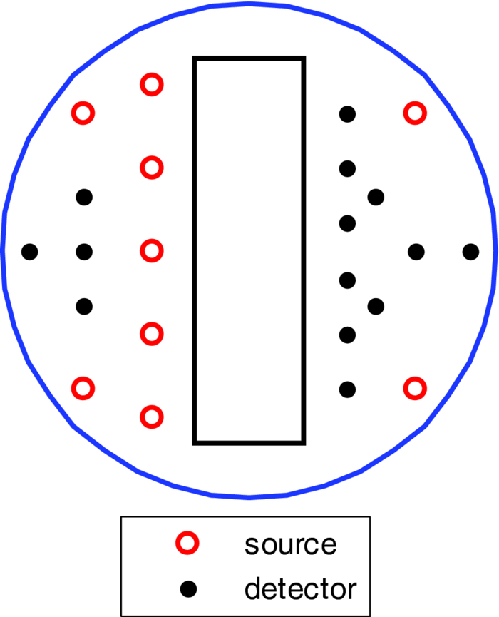

In phantom experiments, the frequency domain system³⁸ consisted of 14 parallel detectors and four laser diodes of wavelength 740, 780, 808, and 830 nm, respectively. Each laser diode was sequentially switched to nine positions on the probe. The central slot on the probe shown in Fig. 1 was used to fit the ultrasound transducer, and the sources and detectors were distributed on both sides. The range of source and detector (s-d) distance is from 1.2 to 7.4 cm. Because of the saturation of photomultiplier tubes for very short s-d separation, the useful s-d range is from 2.5 to 7.4 cm, resulting in 134 amplitude and phase measurements for imaging reconstruction. In principle, more detectors and sources that provide larger s-d distances can be deployed to probe deeper targets, however, the signal to noise ratio of those detectors with s-d distance beyond 7.5 cm is too low.

Polyester resin spheres of calibrated values μ_a = 0.23 cm⁻¹ and [TeX:] $\mu _s^\prime $ $μ_{s}^{'}$ = 5.45 cm⁻¹, and μ_a = 0.07 cm⁻¹ and [TeX:] $\mu _s^\prime $ $μ_{s}^{'}$ = 5.50 cm⁻¹ were used to emulate high-contrast tumors and low-contrast benign lesions. Intralipid solution of μ_a = 0.03 cm⁻¹ and [TeX:] $\mu _s ^\prime $ $μ_{s}^{'}$ = 7.2 cm⁻¹ was used to emulate the background tissue. Note that there is a small difference (1.8 cm⁻¹) in [TeX:] $\mu _s ^\prime $ $μ_{s}^{'}$ between the target and the background. We performed simulations to evaluate the contribution of this difference to reconstructed target μ_a and found that its effect was about 2%, which was negligible. All measurements were made with the target inside the intralipid (target data) and intralipid alone as a reference. The perturbation between the target data and the reference was used for imaging reconstruction.

Clinical experiments were performed at University of Connecticut Health Center. The study protocol was approved by the local Institutional Review Board committee. All patients who participated in our study signed the informed consent. The data were taken at the patients’ lesion area and the contralateral breast of the same quadrant of the lesion. Contralateral data set was used to estimate background optical properties for weight matrix computation. The perturbation computed between the lesion data and the contralateral data was used for imaging reconstruction.

3. Results

3.1.

Two Targets with Different Contrast

In some clinical cases, patients may have multiple lesions with malignant or benign characteristics. To evaluate the performance of our multi-zone ROIs approach, we have performed simulations and experiments by using two targets of the same size but different contrast.

A series of FEM simulations were conducted for two types of targets, one high and one low-contrast absorbers. Both targets had the same diameter of 1.0 cm and were located at the same depth with center-to-center separations of 1.5, 2.0, 2.5, and 3.0 cm, respectively. The depth from the target center to the probe surface varied from 1.0 to 2.5 cm in 0.5 cm increments. Tomography images were shown in six slices at different depths from 0.5 cm to 3.0 cm with 0.5 cm increments. The targets were shown at the corresponding depth. The single ROI and the multi-zone ROIs algorithms were used to reconstruct the images as shown in Fig. 2. In Fig. 2, the separation of the two targets is 2.5 cm and target center depths are 1.0, 1.5, 2.0, and 2.5 cm, respectively. The images in the left column [Figs. 2a, 2c, 2e, 2g] are the reconstructed absorption distributions using the single ROI method and the images in the right column [Figs. 2b, 2d, 2f, 2h] are the reconstruction results using the multi-zone ROIs algorithm. For the single ROI method, the reconstructed maximum absorption value of the high-contrast target was 0.09 cm⁻¹ (36% accuracy), and that of the low-contrast target was 0.04 cm⁻¹ (57%) at the depth of 1.5 cm; but the accuracy could reach 0.17 cm⁻¹ (68%) for the high-contrast target and 0.06 cm⁻¹ (86%) for the low-contrast target when the multi-zone method was used. With respect to target resolving capability, the two targets could not be separated using the single ROI method when they were deeper than 2.0 cm. However, the targets up to 2.5 cm depth could be separated with the guidance of the prior target locations when the multi-zone method was used. Briefly, the average reconstruction accuracy of four target separations of the high-contrast targets using the single ROI method was 36, 38, 35, and 33% at 1.0, 1.5, 2.0, and 2.5 cm center depths, respectively. The average accuracy of the corresponding separations was 63, 67, 58, and 47%, respectively, using the multi-zone method. A 23% average improvement was achieved compared with that obtained using the single ROI method. To further evaluate the performance of the multi-zone method with targets of different contrast, another set of simulations with μ_a = 0.15 cm⁻¹ as the low- contrast target and μ_a = 0.25 cm⁻¹ as the high-contrast target, and [TeX:] $\mu _s ^\prime $ $μ_{s}^{'}$ = 6.0 cm⁻¹ for both was performed. For the single ROI method, the average reconstruction accuracy of four separations was 31, 46, 38, and 22% at 1.0 to 2.5 cm center depths, respectively. The average accuracy was 41, 73, 68, and 44%, respectively, and an average 22% improvement was obtained compared with that using the single ROI method.

Fig. 2

Simulated absorption maps of two targets of different contrast (μ_a = 0.25 cm⁻¹ and μ_a = 0.07 cm⁻¹) separated by 2.5 cm and located at 1.0, 1.5, 2.0, and 2.5 cm depth, respectively, using the single ROI shown in (a), (c), (e), and (g) and the multi-zone method shown in (b), (d), (f), and (h). For each figure part, there were six subfigures reconstructed at different depths marked on the figure title. Each subfigure is a spatial x-y image of 9 cm × 9 cm in spatial dimensions. The rest of the figures consisting of reconstructed absorption maps were displayed with the same dimensions as Fig. 2.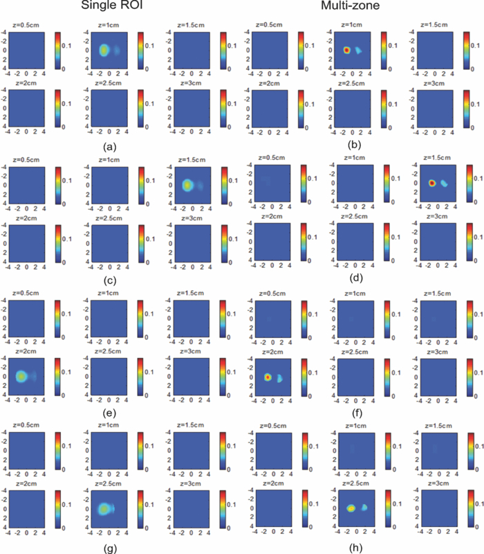

To validate the simulation results, a phantom experiment using two 1-cm polyester resin spheres with different contrasts was performed. The intralipid solution was used as the background. The experiment was designed using similar conditions as the simulation. Figure 3 shows the reconstructed absorption maps of the two targets, which were separated by 2.5 cm and located from 1.0 to 2.5 cm center depths. Targets could not be resolved when they were located deeper than 2.0 cm if the single ROI method was used [Figs. 3e, 3g], while in the right column [Figs. 3b, 3d, 3f, 3h], they could be separated at all depths when the multi-zone method was used. The average accuracy of four target separations of the high-contrast target was 39, 44, 41, and 34% at depths of 1.0, 1.5, 2.0, and 2.5 cm using the single ROI method, respectively, and that was 66, 75, 64, and 56%, respectively, using the multi-zone method. The average improvement was 26%. Both simulations and phantom experiments demonstrated that the multi-zone algorithm could improve the capability of resolving two targets with improved quantification.

Fig. 3

Phantom experimental results of two targets of different contrast (μ_a = 0.23 cm⁻¹ and μ_a = 0.07 cm⁻¹) separated by 2.5 cm and located at 1.0, 1.5, 2.0, and 2.5 cm depth, respectively, using the single ROI shown in (a), (c), (e), and (g) and the multi-zone method shown in (b), (d), (f), and (h).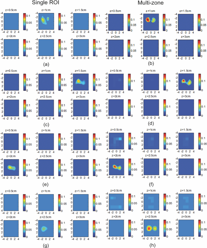

Figure 4 shows the analysis of reconstruction accuracy quantified using accuracy versus different depths. The solid curves are for a high-contrast target using the multi-zone method, while the dotted lines are obtained from the single ROI method. The dashed lines are for the low-contrast target using the multi-zone method. Because of the limited resolving ability of the single ROI method for the low-contrast target, the accuracy could not be accurately measured and therefore no values are given. The 100% is plotted as the reference using the dashed-dotted line. Figures 4a, 4b show the results of the simulations, where Fig. 4a corresponds to the two targets with μ_a = 0.25 cm⁻¹ and μ_a = 0.07 cm⁻¹ and Fig. 4b to μ_a = 0.25 cm⁻¹ and μ_a = 0.15 cm⁻¹. Figure 4c shows the results of the phantom experiments. The improvement of the multi-zone method is shown by its higher reconstruction accuracy (solid lines) than that of the single ROI method (dotted lines). From the comparison between the figures, one can see that the reconstructed absorption values of the high-contrast target remain similar and the most accurate reconstructions occur at the depth range beyond 1.0 cm and less than 2.5 cm. For the low-contrast target (true μ_a = 0.07 cm⁻¹), the reconstruction values were around or slightly over the true value 100% [Figs. 4a, 4c]. For the medium-contrast target (true μ_a = 0.15 cm⁻¹) imaged with the high-contrast target together, both targets were under-reconstructed but the medium-contrast target had higher accuracy than that of the high-contrast target [Fig. 4b].

Fig. 4

Plot of reconstruction accuracy versus target depths of two targets using the single ROI and multi-zone method as labeled in the figures. (a) and (b) From simulations and (c) from experiments. (a) Two targets of μ_a = 0.25 cm⁻¹ and μ_a = 0.07 cm⁻¹; (b) μ_a = 0.25 cm⁻¹ and μ_a = 0.15 cm⁻¹; (c) μ_a = 0.23 cm⁻¹ and μ_a = 0.07 cm⁻¹.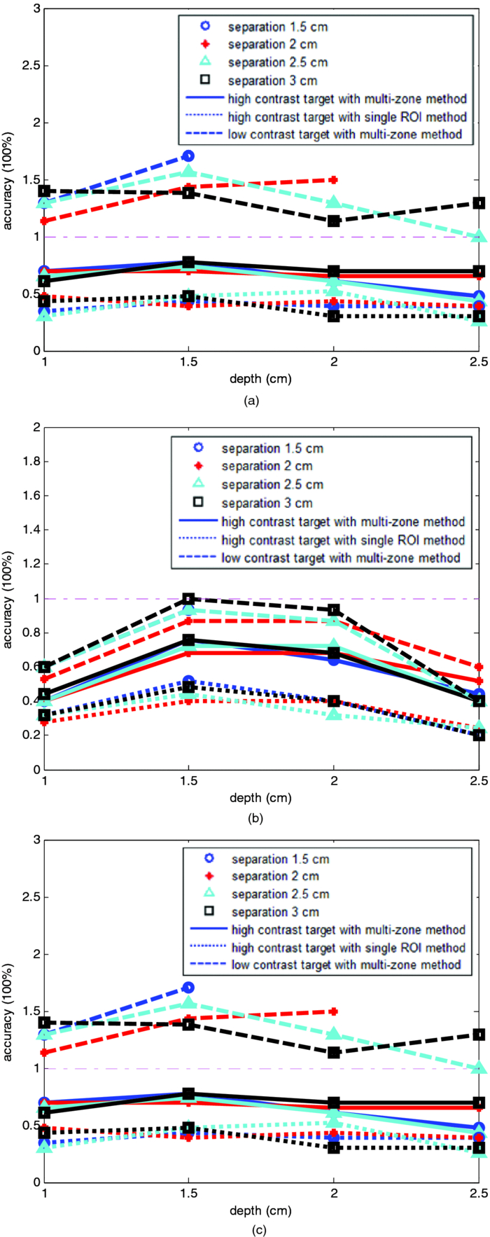

A clinical example was given to demonstrate the improvement by using the multi-zone method. This 52-year old patient had two suspicious lesions as shown in US [Fig. 5a]. When the single ROI was used, two targets of one slightly higher contrast (left) than the other (right) showed in the absorption map reconstructed at 780 nm [Fig. 5b] and 830 nm (not shown). The calculated maximum absorption coefficients were 0.13 and 0.10 cm⁻¹, respectively. When the multi-zone method was used, the calculated maximum absorption coefficients were 0.22 and 0.12 cm⁻¹ [Fig. 5c]. The calculated maximum total hemoglobin (Hb) concentrations were 80 and 63 μmol/Liter by using the single ROI method [Fig. 5d], and 97 and 62 μmol/Liter by using the multi-zone method [Fig. 5e]. Biopsy results showed that the higher contrast lesion was a ductal carcinoma in situ (left in US) and the lower contrast one was a benign fibrocystic lesion.

Fig. 5

A clinical example of two different contrast lesions. (a) Co-registered US showed two suspicious masses with centers located at 1.2 cm from the skin surface. (b) and (c) Optical absorption map reconstructed at 780 nm using the (b) single ROI and (c) multi-zone method. (d) and (e) Computed total hemoglobin concentration map using the (d) single ROI and (e) multi-zone method.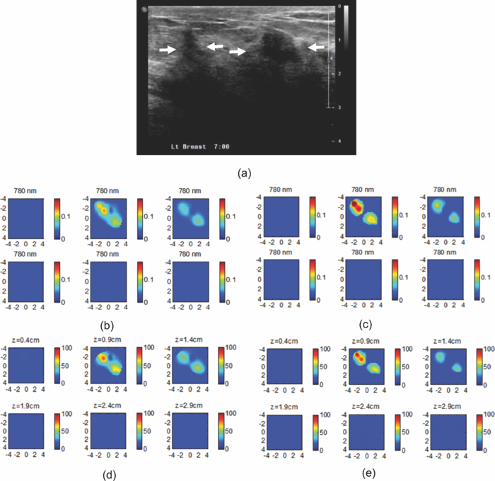

3.2.

Two Targets with the Same Contrast

In this section, the resolving ability of the multi-zone ROIs method in imaging clustered tumors with the same contrast was evaluated using simulations and phantom experiments. Two small targets of 1.0 cm diameter and the same contrast located at the same or different depths were characterized.

In the first set of FEM simulations, two high-contrast targets of 1.0 cm diameter were imaged. The target center-to-center separations were 1.5, 2.0, 2.5, and 3.0 cm, and center depths varied from 1.0 to 2.5 cm. Figure 6 shows an example when the two targets with 2.5 cm separation are located at the same depths from 1.0 to 2.5 cm. A comparison of the results in the left column [Figs. 6a, 6c, 6e, 6g] using the single ROI method and in the right column [Figs. 6b, 6d, 6f, 6h] using the multi-zone method has clearly demonstrated that the capability of the multi-zone method in resolving two targets is much better. Quantitatively, the single ROI method had the best reconstructed absorption value of 0.11 cm⁻¹ (44%) at 1.5 cm depth; and lost the resolving ability when the target was deeper than 2.0 cm. In contrast, the multi-zone method can reach 0.19 cm⁻¹ (76%) reconstruction accuracy and extend resolving ability up to 2.5 cm. The average reconstruction accuracy of four different target separations was 33, 42, 40, and 27% from 1.0 to 2.5 cm center depths, respectively, using the single ROI method. The average accuracy was 45, 74, 60, and 41%, respectively, using the multi-zone method. An average 20% improvement was achieved compared with that using the single ROI method.

Fig. 6

Simulated absorption maps of two targets with the same contrast (μ_a = 0.25 cm⁻¹) separated by 2.5 cm and located at 1.0, 1.5, 2.0, and 2.5 cm depth, respectively. Obtained (a), (c), (e), and (g) using the single ROI and (b), (d), (f), and (h) using the multi-zone method.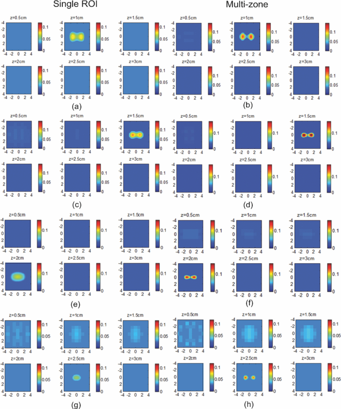

Phantom experiments were performed to verify the simulation results. Two high-contrast phantom targets of 1.0 cm diameter were embedded inside the intralipid solution with the same experimental conditions as the simulation. Figure 7 shows one example of the phantom targets separated by 2.5 cm at all depths. The average reconstruction accuracy was 29, 37, 41, and 28% at 1.0, 1.5, 2.0, and 2.5 cm center depths, respectively, using the single ROI method and the value was 47, 84, 65, and 42%, respectively, using the multi-zone method. An average 26% improvement was achieved compared with that using the single ROI method. Figure 8 plots the accuracy ratio versus different depths. The reconstruction accuracy of the multi-zone method (solid lines) is much higher than that of the single ROI method (dotted lines). The more accurate reconstruction occurred in depth range beyond 1.0 cm and less than 2.5 cm in both simulations [Fig. 8a] and phantom experiments [Fig. 8b].

Fig. 7

Phantom results of two targets with the same contrast (μ_a = 0.23 cm⁻¹) separated by 2.5 cm and located at 1.0, 1.5, 2.0, and 2.5 cm depth, respectively. Obtained (a), (c), (e), and (g) using the single ROI method and (b), (d), (f), and (h) using the multi-zone method.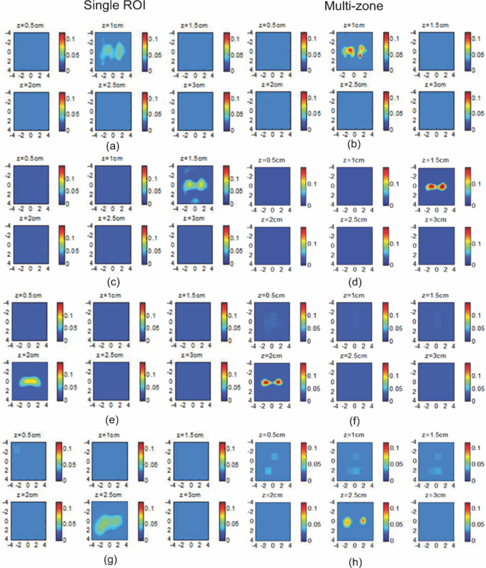

Fig. 8

Plot of reconstruction accuracy versus target depths of two targets of the same contrast. (a) Simulation results of two targets of μ_a = 0.25 cm⁻¹ and (b) phantom results of μ_a = 0.23 cm⁻¹.

The second set of simulations was performed with two targets located at different depths. The two targets were the same as before but one was located at 1.0 cm depth while another was at 1.5 cm. Different center-to-center separations of 1.5, 2.0, 2.5, and 3.0 cm were simulated and shown in Fig. 9. None of the images shown in the left column [Figs. 9a, 9c, 9e, 9g] obtained from the single ROI method could separate the two targets; while the images shown in the right column [Figs. 9b, 9d, 9f, 9h] obtained from the multi-zone method could resolve them when the center-to-center separation was larger than 2.0 cm. The same as in other cases, the reconstructed absorption coefficients were more accurate when the multi-zone method was used. The absorption coefficients were 0.12 (48%), 0.10 (40%), 0.10 (40%), and 0.10 (40%) for 1.5, 2.0, 2.5, and 3.0 cm center-to-center separations, respectively, using the single ROI method; and those were 0.16 (64%), 0.18 (72%), 0.15 (60%), and 0.16 (64%) using the multi-zone method with an average 23% improvement.

Fig. 9

Simulated absorption maps of two targets of the same contrast (μ_a = 0.25 cm⁻¹) separated by 2.5 cm with one located at 1.0 cm and another located at 1.5 cm center depths. (a), (c), (e), and (g) Obtained using the single ROI method and (b), (d), (f) and (h) using the multi-zone method.

To verify the simulation results, phantom experiments were performed using the similar condition as the simulation. Two high-contrast phantom targets of 1.0 cm diameter were located at 1.0 cm and at 1.5 cm center depths. Figure 10 shows the US and the reconstructed images of the two targets separated by 1.5, 2.0, 2.5, and 3.0 cm. The reconstructed absorption coefficients were 0.10 (43%), 0.09 (39%), 0.08 (35%), and 0.09 (39%) for 1.5, 2.0, 2.5, and 3.0 cm center-to-center separations, respectively, using the single ROI method [Figs. 10a, 10c, 10e, 10g]; and those were 0.16 (70%), 0.14 (61%), 0.17 (74%), and 0.15 (65%) using the multi-zone method [Figs. 10b, 10d, 10f, 10h]. An average 29% improvement was achieved compared with that of the single ROI method. When the separation of the two targets was larger than 2.0 cm, the multi-zone reconstruction method could separate them, but the single ROI method could not.

Fig. 10

Phantom experimental results of two targets of the same contrast (μ_a = 0.23 cm⁻¹) separated by 2.5 cm with one located at 1.0 cm and another located at 1.5 cm center depths. Obtained (a), (c), (e) and (g) from the single ROI method and (b), (d), (f) and (h) from the multi-zone method. The corresponding co-registered US images were shown in the first column.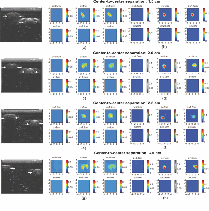

A clinical example with two lesions is given in Fig. 11. A 59-year old woman had two suspicious lesions located at 9 and 7 to 8 o'clock positions. US images of the two lesions are shown in different views in Figs. 11a, 11b with the center depth of approximately 2.0 cm. Because the NIR probe is much bigger (9-cm diameter) than the US probe (5 cm × 1 cm), the two targets are visible in the absorption maps reconstructed using a single ROI at 780 nm [Fig. 11c] and 830 nm (not shown). The calculated maximum absorption coefficients were 0.18 and 0.14 cm⁻¹ for 9 and 7 to 8 o'clock lesions, respectively. When the multi-zone method was used as shown in Fig. 11d, the calculated maximum absorption coefficients were 0.23 and 0.19 cm⁻¹, respectively. The calculated maximum total Hb concentrations were 90 and 81 μ mol/Liter by using the single ROI method, and 105 and 101 μ mol/Liter by using the multi-zone method. Biopsy results showed that both lesions were invasive carcinomas.

Fig. 11

A clinical example of two malignant tumors. (a) and (b) Co-registered US image of 9 o'clock lesion and (b) 7 to 8 o'clock lesion with center location of approximately 2.0 cm. (c) and (d) Absorption maps reconstructed at 780 nm using (c) single ROI, and (d) multi-zone method. (e) and (f) Total hemoglobin concentration maps using (e) single ROI and (f) multi-zone method.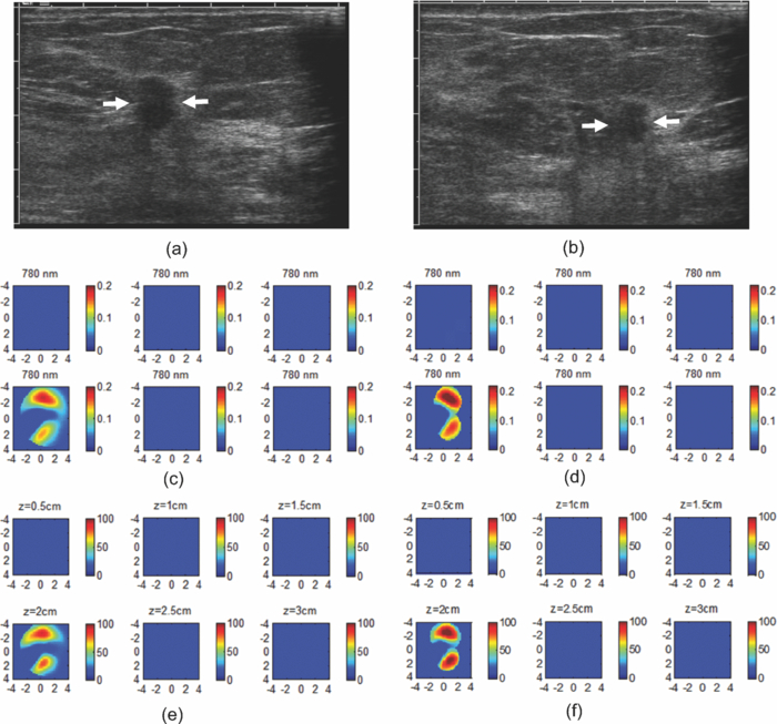

3.3.

Large Target Surrounded by a Small Satellite Target

Large cancers may have smaller satellite lesions in the neighboring areas. To quantify the reconstruction accuracy under this imaging condition, two high-contrast targets of 2 and 1 cm diameter next to each other were simulated using the FEM method. Two sets of simulations were performed where the larger target was surrounded by the smaller one closer to its top half or bottom half in depth. In the first set of simulations, the larger target was located at 1.5 or 2.0 cm center depth and the smaller target located closer to its top half with the center-to-center separation of 2.1, 2.5, 3.0, and 3.5 cm, respectively. Figures 12a, 12b show the absorption maps of the two targets with 3.0 cm separation when the larger one is located at 1.5 cm center depth. The reconstructed maximum absorption of the larger target using the single ROI method [Fig. 12a] was 0.10 cm⁻¹ (40%), and the multi-zone method [Fig. 12b] was 0.16 cm⁻¹ (64%). The smaller target was not resolved using the single ROI method [Fig. 12a] and was 0.09 cm⁻¹ (36%) using the multi-zone method [Fig. 12b]. More results of different target separations and depths are given in Table 1. The average reconstruction accuracy of the larger target was 51.5% and the satellite target could not be resolved until the separation was larger than 3.5 cm if the single ROI method was used. The accuracy of the larger target could reach 78.5% using the multi-zone method and the satellite target was visible when the separation reached 3.0 cm with the average accuracy of 39%. In the second set of simulations, the larger target with the small satellite target closer to its bottom half was simulated with 2.1 to 3.5 cm separations and the center depths of 1.5 and 2.0 cm. The reconstructed absorption maps are shown in Figs. 12c, 12d. Using the single ROI method, the smaller target could not be resolved and the maximum reconstructed μ_a was 0.10 cm⁻¹ (40%) as shown in Fig. 12c. Using the multi-zone method, the reconstructed maximum absorption of the larger target was 0.15 cm⁻¹ (60%) and that of the smaller one was 0.05 cm⁻¹ (20%) [Fig. 12d]. The satellite target is visible in Fig. 12d but reconstruction accuracy (20%) is far lower than that of the larger one. As shown in Table 1, the average reconstruction accuracy of the larger target is 51.5% using the single ROI method and that is 76% using the multi-zone method. The smaller target could not be resolved until the target separation reached 3.5 cm using the single ROI method and it could be resolved when the separation was larger than 3.0 cm with the average accuracy of 23% using the multi-zone method.

Fig. 12

Simulated absorption maps of one larger target with a smaller target closer to its top half [(a) and (b)], and bottom half [(c) and (d)] using single ROI [(a) and (c)] and multi-zone method [(b) and (d)]. The center to center distance between the two targets was 3.0 cm. (The arrow head points to the smaller target.)

Fig. 13

Phantom experiments of one larger target with a smaller target located close to its top half [(a) and (b)], and bottom half [(c) and (d)] using single ROI [(a) and (c)] and multi-zone method [(b) and (d)]. The corresponding co-registered US images were shown in the left column. (The arrow head points to the smaller target.)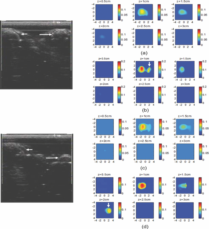

Table 1

Simulation results of reconstructed absorption coefficient and accuracy of one larger target surrounded by a smaller satellite target with the same contrast (μa = 0.25 cm−1) separated by 2.0 to 3.5 cm at 1.0 to 2.5 cm center depth, respectively, using single ROI and multi-zone method.

		Smaller target closer to the top half				Smaller target closer to the bottom half
		Larger target depth 1.5 cm		Larger target depth 2.0 cm		Larger target depth 1.5 cm		Larger target depth 2.0 cm
Reconstructed μa Unit: (cm−1)		Single ROI	Multi-zone	Single ROI	Multi-zone	Single ROI	Multi-zone	Single ROI	Multi-zone
Target separation 2.0 cm	Max(L): Max(S):	(0.11)1 (44%)	(0.16)1 (64%)	(0.16)1 (64%)	(0.23)1 (92%)	(0.11)1 (44%)	(0.17)1 (68%)	(0.16)1 (64%)	(0.22)1 (88%)
Target separation 2.5 cm	Max(L): Max(S):	(0.11)1 (44%)	(0.16)1 (64%)	(0.15)1 (60%)	(0.23)1 (92%)	(0.11)1 (44%)	(0.16)1 (64%)	(0.15)1 (60%)	(0.21)1 (84%)
Target separation 3.0 cm	Max(L): Max(S):	(0.10)1 (40%)	0.16 (64%) 0.09 (36%)	(0.15)1 (60%)	0.24 (96%) 0.10 (40%)	(0.10)1 (40%)	0.15 (60%) 0.05 (20%)	(0.15)1 (60%)	0.21 (84%) 0.05 (20%)
Target separation 3.5 cm	Max(L): Max(S):	0.10 (40%) 0.06 (24%)	0.15 (60%) 0.09 (36%)	0.15 (60%) 0.08 (32%)	0.24 (96%) 0.11 (44%)	0.10 (40%) 0.04 (16%)	0.15 (60%) 0.07 (28%)	0.15 (60%) 0.06 (24%)	0.25 (100%) 0.06 (24%)

^*Two targets merged together as one. Max(L) and Max(S) referred to maximum reconstructed absorption coefficient of larger target and smaller target, respectively.

We also performed phantom experiments using two high-contrast polyester resin spheres. Two sets of experiments were done and the targets were located at the same coordinates as used in the simulation described earlier. The left column of the US images in Fig. 13 shows the locations of the two targets when they are separated by 3.0 cm, and the reconstructed absorption maps are shown in the right column. When the smaller target was closer to the top half of the larger one, the reconstructed maximum μ_a of the larger target was 0.09 cm⁻¹ (39%) using the single ROI method [Fig. 13a] and 0.17 cm⁻¹ (74%) using the multi-zone method [Fig. 13b], and the maximum μ_a was 0.11 cm⁻¹ (48%) in Fig. 13b of the smaller target using the multi-zone method. The reconstructed maximum μ_a was 0.09 cm⁻¹ (39%) in Fig. 13c using the single ROI method and 0.16 cm⁻¹ (70%) of the larger target, and 0.11 cm⁻¹ (48%) of the smaller one in Fig. 13d using the multi-zone method when the smaller target was located closer to the bottom half of the larger one. The smaller target cannot be resolved in both Figs. 13a, 13c. In Table 2, the average reconstruction accuracy at all separations and depths is 46.7 and 80.5% (larger target) and 26 and 48% (smaller target) using the single ROI method and the multi-zone method, respectively, when the smaller target is closer to the top half of the larger one. The average values are 49 and 78% (larger target) and 24 and 36% (smaller target) when the smaller target is closer to the bottom half of the larger one. This set of simulations and phantom experiments

Table 2

Phantom experimental results of absorption coefficient and accuracy of one larger target surrounded by a smaller satellite target of the same contrast (μa = 0.25 cm−1) separated by 2.0 to 3.5 cm at 1.0 to 2.5 cm center depth, respectively, using single ROI and multi-zone method.

		Smaller target closer to the top half				Smaller target closer to the bottom half
		Larger target depth 1.5 cm		Larger target depth 2.0 cm		Larger target depth 1.5 cm		Larger target depth 2.0 cm
Reconstructed μa Unit (cm−1)		Single ROI	Multi-zone	Single ROI	Multi-zone	Single ROI	Multi-zone	Single ROI	Multi-zone
Target separation 2.0 cm	Max(L): Max(S):	(0.08)1 (35%)	(0.12)1 (52%)	(0.10)1 (43%)	(0.16)1 (70%)	(0.10)1 (43%)	(0.13)1 (57%)	(0.13)1 (57%)	(0.17)1 (74%)
Target separation 2.5 cm	Max(L): Max(S):	(0.10)1 (43%)	(0.19)1 (83%)	(0.14)1 (61%)	(0.23)1 (100%)	(0.09)1 (39%)	(0.16)1 (70%)	(0.13)1 (57%)	(0.23)1 (100%)
Target separation 3.0 cm	Max(L): Max(S):	(0.09)1 (39%)	0.17 (74%) 0.11 (48%)	(0.13)1 (57%)	0.23 (100%) 0.11 (48%)	(0.09)1 (39%)	0.16 (70%) 0.11 (48%)	(0.14)1 (61%)	0.23 (100%) 0.05 (22%)
Target separation 3.5 cm	Max(L): Max(S):	0.09 (39%) 0.06 (26%)	0.15 (65%) 0.11 (48%)	0.13 (57%) 0.06 (26%)	0.23 (100%) 0.11 (48%)	0.09 (39%) 0.05 (22%)	0.15 (65%) 0.11 (48%)	0.13 (57%) 0.06 (26%)	0.21 (91%) 0.06 (26%)

^*Two targets merged together as one. Max(L) and Max(S) referred to maximum reconstructed absorption coefficient of larger target and smaller target, respectively.

demonstrated the improvement and limitations when the clustered lesions of different sizes were imaged by the multi-zone algorithm.

4. Discussion and Summary

We have qualitatively evaluated the performance of the single ROI reconstruction method and the new multi-zone reconstruction method with respect to the resolving ability and light quantification accuracy when multiple targets were present. In general, the single ROI method cannot resolve two small targets when their separations were less than 2.5 cm and the target depth was greater than 2.0 cm. The highest reconstruction accuracy of the single ROI method for small dual targets was about 50% for high-contrast targets. The multi-zone reconstruction method improved both the resolving ability and accuracy when the a priori lesion location information was given. As a result, two targets located at 2.5 cm depth with separation greater than 2.0 cm could be distinguished. With respect to light quantification at all depths and separations, the multi-zone method improved the accuracy and the highest reconstruction could reach 91% for high-contrast targets.

Due to the intense light scattering in a turbid medium, the light quantification of targets located at deeper depths of more than 2.5 cm was lower and the resolving capability of the multiple targets was poorer. In addition, because the diffusion approximation was used in reconstruction and the lacking of the center source, targets located at a shallower depth were not as accurately quantified as the targets located beyond 1.0 and less than 2.5 cm depth range. The multi-zone method improved the light quantification for smaller 1-cm dual targets of different separations located at all depths and the improvement was more dramatic when targets were in the depth range beyond 1.0 cm and less than 2.5 cm. Another issue is related to the reconstruction accuracy of different contrast targets. In this paper, we have three sets of targets that have high (0.25 cm⁻¹), medium (0.15 cm⁻¹), and low contrast (0.07 cm⁻¹). Over-reconstruction happened to the low-contrast target due to system and measurement noise and under-reconstruction occurred to high- and medium-targets, however, medium-contrast targets had higher reconstruction accuracy than that of high-contrast targets because of the use of the linear Born approximation. In clinical studies, multiple lesions located close to each other is not uncommon, a diagnostic modality should be able to more accurately characterize multiple lesions. In all simulations and phantom experiments, the multi-zone method achieved more than 20% improvement compared to that of the single ROI method. Thus, it is more accurate in diagnosis of clustered lesions. Further improvement is needed by investigating the use of nonlinear reconstruction algorithms.

When two targets of the same contrast, one larger and one smaller, were located close to each other, the location of the reconstructed absorption mass was shifted toward the larger target because the perturbation generated by the larger target dominated the reconstruction. A smaller target located more than 3 cm away from the larger one may be resolved when the multi-zone algorithm is used, however, the reconstruction accuracy was low. Therefore, it is not reliable to use the multi-zone method to characterize the clustered lesions with a primary larger tumor that dominates the reconstruction. In other words, when the primary tumor is malignant, the smaller lesions around it cannot be correctly diagnosed using the diffused optical tomography even with a priori target information.

In summary, we have introduced a new multi-zone reconstruction method and compared its performance with the single ROI method. Simulation and phantom studies have showed a more than 20% improvement in target quantification as compared to that of the single ROI method. Clinical examples were given to demonstrate the potential of the new method in accurate characterization of malignant and benign breast lesions.

Acknowledgments

This work has been supported by the National Institute of Health (R01EB002136) and the Donaghue Medical Research Foundation.

References

1.

B. J. Tromberg, A. Cerussi, N. Shah, M. Compton, A. Durkin, D. Hsiang, J. Butler, and R. Mehta, “Imaging in breast cancer: diffuse optics in breast cancer: detecting tumors in pre-menopausal women and monitoring neoadjuvant chemotherapy,” Breast Cancer Res. Treat., 7 (6), 279 –285 (2005). Google Scholar

2.

D. R. Leff, O. J. Warren, L. C. Enfield, A. Gibson, T. Athanasiou, D. K. Patten, J. Hebden, G. Z. Yang, and A. Darzi, “Diffuse optical imaging of the healthy and diseased breast: a systematic review,” Breast Cancer Res. Treat., 108 (1), 9 –22 (2008). https://doi.org/10.1007/s10549-007-9582-z Google Scholar

3.

B. Chance, S. Nioka, J. Zhang, E. F. Conant, E. Hwang, S. Briest, S. G. Orel, M. D. Schnall, and B. J. Czerniecki, “Breast cancer detection based on incremental biochemical and physiological properties of breast cancers: a six-year, two-site study,” Acad. Radiol., 12 925 –933 (2005). https://doi.org/10.1016/j.acra.2005.04.016 Google Scholar

4.

J. Wang, S. Jiang, Z. Li, R. M. diFlorio-Alexander, R. J. Barth, P. A. Kaufman, B. W. Pogue, and K. D. Paulsen, “In vivo quantitative imaging of normal and cancerous breast tissue using broadband diffuse optical tomography,” Med. Phys., 37 (7), 3715 –3724 (2010). https://doi.org/10.1118/1.3455702 Google Scholar

5.

S. P. Poplack, T. D. Tosteson, W. A. Wells, B. W. Pogue, P. M. Meaney, A. Hartov, C. A. Kogel, S. K. Soho, J. J. Gibson, and K. D. Paulsen, “Electromagnetic breast imaging: results of a pilot study in women with abnormal mammograms,” Radiology, 243 350 –359 (2007). https://doi.org/10.1148/radiol.2432060286 Google Scholar

6.

R. Choe, A. Corlu, K. Lee, T. Durduran, S. D. Konecky, M. Grosicka-Koptyra, S. R. Arridge, B. J. Czerniecki, D. L. Fraker, A. Demichele, B. Chance, M. A. Rosen, and A. G. Yodh, “Diffuse optical tomography of breast cancer during neoadjuvant chemotherapy: a case study with comparison to MRI,” Med. Phys., 32 1128 –1139 (2005). https://doi.org/10.1118/1.1869612 Google Scholar

7.

X. Liang, Q. Zhang, C. Li, S. R. Grobmyer, L. L. Fajardo, and H. B. Jiang, “Phase-contrast diffuse optical tomography1: pilot results in the Breast,” Acad Radiol., 15 (7), 859 –866 (2008). https://doi.org/10.1016/j.acra.2008.01.028 Google Scholar

8.

X. Intes, “Time-domain optical mammography SoftScan: initial results,” Acad Radiol., 12 (8), 934 –947 (2005). https://doi.org/10.1016/j.acra.2005.05.006 Google Scholar

9.

L. Spinelli, A. Torricelli, A. Pifferi, P. Taroni, G. Danesini, and R. Cubeddu, “Characterization of female breast lesions from multiwavelength time-resolved optical mammography,” Phys. Med. Biol., 50 2489 –2502 (2005). https://doi.org/10.1088/0031-9155/50/11/004 Google Scholar

10.

C. H. Schmitz, D. P. Klemer, R. Hardin, M. S. Katz, Y. Pei, H. L. Graber, M. B. Levin, R. D. Levina, N. A. Franco, W. B. Solomon, and R. L. Barbour, “Design and implementation of dynamic near-infrared optical tomographic imaging instrumentation for simultaneous dual-breast measurements,” Appl. Opt., 44 2140 –2153 (2005). https://doi.org/10.1364/AO.44.002140 Google Scholar

11.

L. S. Fournier, D. Vanel, A. Athanasiou, W. Gatzemeier, I. V. Masuykov, A. R. Padhani, C. Dromain, K. Galetti, R. Sigal, A. Costa, and C. Balleyguier, “Dynamic optical breast imaging: a novel technique to detect and characterize tumor vessels,” Eur. J. Radiol., 69 43 –49 (2009). https://doi.org/10.1016/j.ejrad.2008.07.038 Google Scholar

12.

D. Floery, T. H. Helbich, C. C. Riedl, S. Jaromi, M. Weber, S. Leodolter, and M. H. Fuchsjaeger, “Characterization of benign and malignant breast lesions with computed tomographic laser mammography (CTLM),” Invest. Radiol., 40 328 –335 (2005). https://doi.org/10.1097/01.rli.0000164487.60548.28 Google Scholar

13.

D. Grosenick, H. Wabnitz, K. T. Moesta, J. Mucke, P. M. Schlag, and H. Rinneberg, “Time-domain scanning optical mammography: II. Optical properties and tissue parameters of 87 carcinomas,” Phys. Med. Biol., 50 (11), 2451 –2468 (2005). https://doi.org/10.1088/0031-9155/50/11/002 Google Scholar

14.

B. Brooksby, B. W. Pogue, S. Jiang, H. Dehghani, S. Srinivasan, C. Kogel, T. D. Tosteson, J. Weaver, S. P. Poplack, and K. D. Paulsen, “Imaging breast adipose and fibroglandular tissue molecular signatures by using hybrid MRI-guided near-infrared spectral tomography,” Proc. Natl. Acad. Sci. U.S.A., 103 8828 –8833 (2006). https://doi.org/10.1073/pnas.0509636103 Google Scholar

15.

H. R. Ghadyani, S. Srinivasan, B. W. Pogue, and K. D. Paulsen, “Characterizing accuracy of total hemoglobin recovery using contrast-detail analysis in 3D image-guided near infrared spectroscopy with the boundary element method,” Opt. Express, 18 (15), 15917 –15935 (2010). https://doi.org/10.1364/OE.18.015917 Google Scholar

16.

H. Soliman, A. Gunasekara, M. Rycroft, J. Zubovits, R. Dent, J. Spayne, M. J. Yaffe, and G. J. Czarnota, “Functional imaging using diffuse optical spectroscopy of neoadjuvant chemotherapy response in women with locally advanced breast cancer,” Clin. Cancer Res., 16 (9), 2605 –2614 (2010). https://doi.org/10.1158/1078-0432.CCR-09-1510 Google Scholar

17.

Q. Zhu, P. Hegde, A. Ricci, M. Kane, A. Cronin, Y. Ardeshirpour, C. Xu, A. Aguirre, S. Kurtzman, P. Deckers, and S. Tannenbaum, “The potential role of optical tomography with ultrasound localization in assisting ultrasound diagnosis of early-stage invasive breast cancers,” Radiology, 256 (2), 367 –378 (2010). https://doi.org/10.1148/radiol.10091237 Google Scholar

18.

Q. Zhu, S. Tannenbaum, P. Hegde, M. Kane, C. Xu, and S. H. Kurtzman, “Noninvasive monitoring of breast cancer during neoadjuvant chemotherapy using optical tomography with ultrasound localization,” Neoplasia, 10 (10), 1028 –1040 (2008). Google Scholar

19.

A. Cerussi, D. Hsiang, N. Shah, R. Mehta, A. Durkin, J. Butler, and B. J. Tromberg, “Predicting response to breast cancer neoadjuvant chemotherapy using diffuse optical spectroscopy,” Proc. Natl. Acad. Sci. U.S.A., 104 4014 –4019 (2007). https://doi.org/10.1073/pnas.0611058104 Google Scholar

20.

S. Jiang, B. Pogue, C. Carpenter, S. Poplack, W. Wells, C. Kogel, J. Forero, L. Muffly, G. Schwartz, K. Paulsen, and P. Kaufman, “Evaluation of breast tumor response to neoadjuvant chemotherapy with tomographic diffuse optical spectroscopy: case studies of tumor region-of-interest changes,” Radiology, 252 551 –560 (2009). https://doi.org/10.1148/radiol.2522081202 Google Scholar

21.

C. Zhou, R. Choe, N. Shah, T. Durduran, G. Yu, A. Durkin, D. Hsiang, R. Mehta, J. Butler, A. Cerussi, B. J. Tromberg, and A. G. Yodh, “Diffuse optical monitoring of blood flow and oxygenation in human breast cancer during early stages of neoadjuvant chemotherapy,” J. Biomed. Opt., 12 (5), 051903 (2007). https://doi.org/10.1117/1.2798595 Google Scholar

22.

Q. Zhang, T. J. Brukilacchio, A. Li, J. J. Stott, T. Chaves, E. Hillman, T. Wu, M. A. Chorlton, E. Rafferty, R. H. Moore, D. B. Kopans, and D. A. Boas, “Coregistered tomographic x-ray and optical breast imaging: initial results,” J. Biomed. Opt., 10 1 –9 (2005). Google Scholar

23.

Q. Fang, J. Selb, S. A. Carp, G. Boverman, E. L. Miller, D. H. Brooks, R. H. Moore, D. B. Kopans, and D. A. Boas, “Combined optical and x-ray tomosynthesis breast imaging,” Radiology, 258 (1), 89 –97 (2011). https://doi.org/10.1148/radiol.10082176 Google Scholar

24.

Z. Yuan, Q. Z. Zhang, E. S. Sobel, and H. B. Jiang, “Tomographic x-ray-giuided three dimensional diffuse optical tomography of osteoarthritis in the finger joints,” J. Biomed. Opt., 13 (4), 044006 (2008). https://doi.org/10.1117/1.2965547 Google Scholar

25.

Q. Zhu, E. B. Cronin, A. A. Currier, H. S. Vine, M. M. Huang, N. G. Chen, and C. Xu, “Benign versus malignant breast masses: optical differentiation with US-guided optical imaging reconstruction,” Radiology, 237 57 –66 (2005). https://doi.org/10.1148/radiol.2371041236 Google Scholar

26.

Q. Fang, S. A. Carp, J. Selb, G. Boverman, Q. Zhang, D. B. Kopans, R. H. Moore, E. L. Miller, D. H. Brooks, and D. A. Boas, “Combined optical imaging and mammography of the healthy breast: optical contrast derived from breast structure and compression,” IEEE Trans. Med. Imaging, 28 (1), 30 –42 (2009). https://doi.org/10.1109/TMI.2008.925082 Google Scholar

27.

Q. Zhu, S. Tannenbaum, and S. Kurtzman, “Optical tomography with ultrasound localization for breast cancer diagnosis and treatment monitoring,” Surg. Oncol. Clin. N. Am., 16 (2), 307 –321 (2007). https://doi.org/10.1016/j.soc.2007.03.008 Google Scholar

28.

Q. Zhu, S. Kurtzman, P. Hegde, S. Tannenbaum, M. Kane, M. M. Huang, N. G. Chen, B. Jagjivan, and K. Zarfos, “Utilizing optical tomography with ultrasound localization to image heterogeneous hemoglobin distribution in large breast cancers,” Neoplasia, 7 (3), 263 –270 (2005). https://doi.org/10.1593/neo.04526 Google Scholar

29.

Q. Zhu, C. Xu, P. Guo, A. Aguirre, B. Yuan, F. Huang, D. Castilo, J. Gamelin, S. Tannenbaum, M. Kane, P. Hegde, and S. Kurtzman, “Optimal probing of optical contrast of breast lesions of different size located at different depths by US localization,” Technol. Cancer Res. Treat., 5 (4), 365 –380 (2006). Google Scholar

30.

F. H. Tian, H. J. Niu, S. Khadka, Z. J. Lin, and H. L. Liu, “Algorithmic depth compensation improves quantification and noise suppression in functional diffuse optical tomography,” Biomed. Opt. Express, 1 (2), 441 –452 (2010). https://doi.org/10.1364/BOE.1.000441 Google Scholar

31.

H. J. Niu, Z. J. Lin, F. H. Tian, S. Dhamne, and H. L. Liu, “Comprehensive investigation of three dimensional diffuse optical tomography with depth compensation algorithm,” J. Biomed. Opt., 15 (4), 046005 (2010). https://doi.org/10.1117/1.3462986 Google Scholar

32.

Q. Zhu, N. G. Chen, and S. Kurtzman, “Imaging tumor angiogenesis using combined near infrared diffusive light and ultrasound,” Opt. Lett., 28 337 –339 (2003). https://doi.org/10.1364/OL.28.000337 Google Scholar

33.

H. Jiang, K. Paulsen, U. Osterberg, and M. Patterson, “Frequency-domain near-infrared photo diffusion imaging: initial evaluation in multitarget tissuelike phantoms,” Med. Phys., 25 183 –193 (1998). https://doi.org/10.1118/1.598179 Google Scholar

34.

S. C. Davis, H. Dehghani, P. K. Yalavarthy, B. W. Pogue, and K. D. Paulsen, “Comparing two regularization techniques for diffuse optical tomography,” Proc. SPIE, 6434 64340X (2007). https://doi.org/10.1117/12.700364 Google Scholar

35.

H. L. Graber, Y. Xu, and R. L. Barbour, “Image correction scheme applied to functional diffuse optical tomography scattering images,” Appl. Opt., 46 (10), 1705 –1716 (2007). https://doi.org/10.1364/AO.46.001705 Google Scholar

36.

F. Yang, F. Gao, P. Q. Ruan, and H. J. Zhao, “Combined domain-decomposition and matrix-decomposition scheme for large-scale diffuse optical tomography,” Appl. Opt., 49 (16), 3111 –3126 (2010). https://doi.org/10.1364/AO.49.003111 Google Scholar

37.

M. M. Huang, T. Q. Xie, G. Chen, and Q. Zhu, “Simultaneous reconstruction of absorption and scattering maps with ultrasound localization: feasibility study using transmission geometry,” Appl. Opt., 42 (19), 4102 –4114 (2003). https://doi.org/10.1364/AO.42.004102 Google Scholar

38.

Y. Ardeshirpour, M. M. Huang, and Q. Zhu, “Effect of the chest wall on breast lesion reconstruction,” J. Biomed Opt., 14 (4), 044005 (2009). https://doi.org/10.1117/1.3160548 Google Scholar

39.

T. Durduran, R. Choe, J. P. Culver, L. Zubkov, M. J. Holboke, J. Giammarco, B. Chance, and A. G. Yodh, “Bulk optical properties of healthy female breast tissue,” Phys. Med. Biol., 47 2847 –2861 (2002). https://doi.org/10.1088/0031-9155/47/16/302 Google Scholar

Citation Download Citation

Yan Xu, Chen Xu, and Quing Zhu "Clustered targets imaged by optical tomography guided by ultrasound," Journal of Biomedical Optics 16(7), 076018 (1 July 2011). https://doi.org/10.1117/1.3600773

Published: 1 July 2011

Access the abstract

JOURNAL ARTICLE
17 PAGES

DOWNLOAD PAPER SAVE TO MY LIBRARY

GET CITATION

CITATIONS

Cited by 2 scholarly publications.

Explore citations on Lens.org

RIGHTS & PERMISSIONS

Get copyright permission Get copyright permission on Copyright Marketplace

KEYWORDS

Absorption

Target designation

Ultrasonography

Optical tomography

Reconstruction algorithms

Satellites

Sensors

1.

Introduction

2.

Methods