The use of spectra in the identification and characterization of biological and chemical substances is constantly growing as the different measurement techniques are simplified and commercialized. The expansion from detecting a single spectrum from one point in the sample to measuring spectra for every pixel with a hyperspectral camera has opened the door to a lot of new applications. It has not yet reached its full potential, though it is used extensively in remote sensing, and it is now becoming part of commercial imaging setups for biomedical applications. In particular, the use of hyperspectral imaging in confocal microscopes (for example, the Zeiss META system) in microscopic analysis as classification in fluorescence in situ hybridization (FISH)¹ and fluorescence microscopes has emerged. With this availability, the need for good methods for analyzing the large data sets (known as hyperspectral cubes) is apparent. Common ways of doing this analysis is by using principle component analysis (PCA)² or linear spectral unmixing.³ In remote sensing, there has also been some usage of spectral mixture analysis⁴ and spectral angle mapping,⁵ as compared by Dennison et al.⁶

PCA works on the full hyperspectral cube without making assumptions about the sample, and it projects the spectral data into a new orthogonal basis, where the axes are computed with respect to the largest spread in the spectral data between pixels. In comparison, spectral unmixing works individually on each pixel and assumes that the resulting spectrum in a pixel is a linear combination of a set of reference spectra, and solves for the amount of each reference spectra using linear algebra. These techniques are straightforward and work well for samples with high signal-to-noise ratios and small effects from interfering background signals.

We use the data from individual pixels in the image, just as in the case of linear unmixing, but the analysis is based on the correlation coefficient⁷

where $X$ and $Y$ are random variables, ${\sigma }_{XY}$ is the covariance between $X$ and $Y$, and ${\sigma }_X$, ${\sigma }_Y$ is the standard deviation for $X$ and $Y$, respectively. The correlation coefficient is scale-free, meaning that it is independent of the units of measure for $X$ and $Y$. Its resulting value will be in the interval $-1\le {\rho }_{XY}\le 1$, where 1 corresponds to $(Y=X)$ and $-1$ to $Y=-X$. In the case of hyperspectral data, the variables $X$ and $Y$ are the two spectra (one from the image and one from the reference) with $N$ data points each, and the correlation coefficient (which will be called correlation from now on) is, then, given by where $\overline{X}$, $\overline{Y}$ are the mean values of $X$ and $Y$.

This method is robust with respect to noise, and it has been used for decades in remote sensing applications such as radar, where it can recover signals with signal-to-noise values of less than 1.^8,9 Since the signal-to-noise ratio in hyperspectral data can be low, due to the total intensity being separated into numerous wavelength channels, the use of correlation is favorable on such signals.

As an application of the correlation analysis, a 379-day-old male APP/PS1 mouse was injected with the well-known luminescent conjugated oligothiophene (LCO) pFTAA,^10–12 which is known to bind to amyloid $\beta$ plaques in the brain that are known to be related to the progression of Alzheimer’s disease.^10–12 Specifically, APP/PS1 mice were given two consecutive injections of pFTAA [or PBS for a reference autofluorescence (AF) spectrum] and were sacrificed 24 h after the second injection. The brain was snap-frozen, and 30 μm cryo sections were prepared. These sections were fixed in ethanol, rehydrated with PBS, and mounted with Dako fluorescence mounting medium (Dako Cytomation, Glostrup, Denmark).

In addition, a reference brain section from a 174-day-old female APP/PS1 mouse was injected with PBS buffer and used as reference for the AF. Both of these were imaged using a Carl Zeiss AG LSM 510 META system with a laser excitation of 800 nm. This excitation ensured 2-photon absorption at 400 nm in the sample, yielding visible fluorescence from the pFTAA as well as the AF. The oligothiophene pFTAA and other related polymer analogs, such as PTAA, are known to have an appreciable 2-photon absorption cross section at 800 nm.¹³ The fluorescence was then recorded into a spectrum for every pixel by the attached multichannel META detector. These pixels were then put together into a hyperspectral image. By acquiring such images for both the pFTAA and PBS sections, the correlation analysis could be done on the pFTAA brain section. The reference spectrum for the AF was found by imaging 10 plaques at an excitation wavelength of 800 nm, selecting the average spectrum of a circle with a diameter of 20 pixels in the central area of the plaques, and then averaging the 10 spectra into a reference spectrum. The pFTAA spectrum was defined from an average over a small region in the center of the plaque of the stained sample. An analysis was then done by calculating two different correlation coefficients between the measured spectra and the reference spectra of the stained sample. These correlation coefficient (from now on known as the correlation) images are shown in Fig. 1.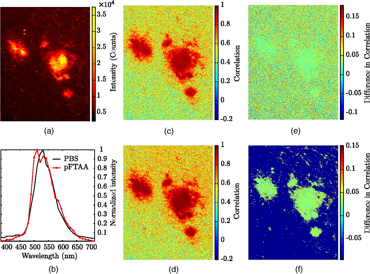

The intensity of the image is shown in Fig. 1(a), and the two reference spectra for AF and the stain pFTAA are shown in Fig. 1(b). Figure. 1(c) and 1(d) displays the map of the correlation between the PBS $({\rho }_{\mathrm{PBS}})$ and pFTAA $({\rho }_{\mathrm{pFTAA}})$ of the stained sample data set, respectively. The last two figures, 1(e) and 1(f), show the difference ${\rho }_{\mathrm{pFTAA}}-{\rho }_{\mathrm{PBS}}$ without thresholding on the intensity (e) and with a threshold of 6,000 counts (f).

As can be seen from the reference spectra, the two spectra are very similar, confirmed by calculating the correlation between them, which is 0.9715. Even though they are this similar and give a high correlation in the plaque, as seen in Fig. 1(c) and 1(d), there is a significant difference between them, shown in Fig. 1(e) and even more clearly in Fig. 1(f), with $({\rho }_{\mathrm{pFTAA}})$ being larger than ${\rho }_{\mathrm{PBS}}$ by approximately 0.04 for the whole plaque.

With the thresholding, we obtain a visually clearer mapping of the excess of the pFTTA signal, as shown in Fig. 1(f). As shown in this image, the method is good at distinguishing one reference spectrum from the background and/or AF, even though the method is well suited for analyzing more than one stain at a time, particularly when the stains have similar fluorescence spectra. In addition, it is not necessary to know more than one of the spectra present, as the correlation gives a statistical number of how similar the spectra are. This makes it possible to statistically compare different images, regardless of their difference in intensity due to factors such as different acquisition settings. Such applications will be tested and validated in forthcoming studies.

The example application of the correlation method on a brain section from an APP/PS1-mouse shows its ability to distinguish two or more similar spectra, including the AF. The method shows promising results for hyperspectral fluorescence and confocal images. It is especially good with noisy images due to the nature of the correlation. However, due to its form, it is best suited for use on spectra where only some of the contributing signals (such as reference spectra) are known.