
|
|
1.IntroductionBy exploiting the penetration depth of light in the classical “therapeutic window” (ranging from 600 to 900 nm), near-infrared (NIR) diffuse optical imaging technique allows the observation of living tissues. This optical imaging technique has gained attention over the past years1–4 because it allows the study of gene expression, protein function and interactions, and a large number of cellular processes. As this technique is sensitive to scattering and absorption variations, it is possible to take advantage of these optical properties to get functional and structural information with simple components (light sources and detectors) for a low cost. Functional imaging in diffuse media was made possible by the development of fluorescent probes emitting in the NIR.5–7 Planar imaging is the simplest way to image the fluorescence; it consists of illuminating the medium with an expanded beam and detecting the outgoing signal with an area detector such as a charged-coupled device (CCD).8,9 It can be performed either in transillumination mode, where the light is shone through the object studied and the transmitted light is then detected on the opposite side, or in epi-illumination mode, where the light is shone from the same side as the backemitted light. For human in vivo imaging, the choice between the transillumination mode and the epi-illumination mode [which is referred to as fluorescence reflectance imaging (FRI)] depends on the depth of the fluorescent target and its location in the body. For example, for breast cancer imaging, transillumination is mostly used. However, for image-guided surgery applications where transillumination is challenging, FRI will be preferred. As we want to target image-guided surgery applications that do not require quantification, we will focus on epi-illumination. We will now discuss the advantages and drawbacks of classical FRI imaging systems. FRI presents several advantages: it offers good sensitivity when the objects observed are close to the surface, is generally fast (acquisition times typically range from a fraction of a second to minutes), and the implementations are easy, low cost, and compact.9,10 On the other hand, this technique suffers from major limitations. The main limitation is the low resolution of the signals detected due to the large scattering of the photons propagated inside the tissue. Because the signal-to-background ratio is a major factor in fluorescence imaging, the other limitation is linked to the background noise caused by excitation leaks, nonspecific fluorescence from injected fluorophores, and/or fluorescence from superficial layers. Contrary to the visible spectrum,11 endogenous sources of fluorescence emit a signal that can be considered negligible in terms of intensity compared with the signal of NIR fluorescence probes in the NIR spectrum, allowing the contrast to be much better as long as the target studied is not located too deeply inside the tissue. However, as the amount of fluorophore bound on a target is generally low,12 the natural fluorescence of tissues coupled to the other parasite signals (excitation leaks, nonspecific fluorescence, or fluorescence from the diet13–15) can then become an obstacle and lead to a limited depth of study: the background signal, even if relatively weak, remains the same while the fluorescence of interest decreases exponentially with depth. Several techniques are used to tackle the low resolution of planar imaging. For example, fluorescence diffuse optical tomography (FDOT)16–21 is aimed at reconstructing the three-dimensional (3-D) localization of fluorophores inside the medium studied. The FDOT method consists of illuminating the medium at several different locations with point sources and detecting the outgoing signals from several different detection points. By using a mathematical model to describe the propagation of photons inside the medium, it is possible to build a 3-D representation of the fluorescence inside the medium. Structured light-based approaches can also be used for FDOT.22 Another way to improve the contrast and resolution is structured illumination. This technique was first applied in microscopy23–26 to obtain a quasi-confocal resolution while still observing a large field of view. It consists of illuminating the sample with sinusoidal patterns at a given spatial frequency. The modulation is effective only in the focal plane of the microscope and the grid disappears with defocus. By acquiring three images at three offset phases and using the proper demodulation formula, it is then possible to obtain the image of the focal plane with a quasi-confocal resolution. This was also applied in the context of diffuse optics with the name spatial frequency domain imaging (SFDI). In this case, the technique relies on the fact that the depth of penetration of light depends on the spatial frequency of the illumination pattern: the smaller the frequency, the deeper the penetration. The acquisition protocol is similar to the one used in microscopy. This technique can be applied to recover the absorption and scattering properties of tissue by fitting the demodulated signals to a light transport model for each pixel on a CCD array,27 but it is also possible to apply it in fluorescence imaging to enhance the signals coming from objects close to the surface by eliminating the signals coming from the deeper layers.28 The technique also allows tomographic reconstruction of absorption contrast by using the analytic inversion equation.29 While SFDI techniques have the advantage of quickly imaging a large field of view, they are only able to select fluorescent signals close to the surface. We propose, in this article, an illumination and detection method that allows us to be more sensitive to certain layers within the tissue (not necessarily close to the surface) by selecting photons, which leads to a reduction of the negative effects on imaging of background signals and scattering. This novel method consists of illuminating the medium with a laser line that scans the area of study and acquiring the images at each position of the illumination line. This line scanning approach (referred to as LS-FRI) gives us access to a stack of images containing more information. This information can be filtered by selecting only specific detection stripes located at a certain distance from the excitation line, the optimal distance depending on the depth of the fluorescent target. We will also show how the remaining information can be used to get an insight on the background signal to be suppressed and can be subtracted from the detected stripe. The proposed method allows us to obtain a better contrast between the fluorescence signal and the background and improves the lateral resolution. In the first part, we will describe the setup used for the study and explain the processing performed on the stack of images acquired. We will then present the results on different cases (a phantom with a single fluorescent inclusion, a fluorescent resolution target, and a phantom with four inclusions at different depths) and prove that this method improves both the contrast and the resolution. We will also show preliminary in vivo results which validate the interest of these methods compared with the classical FRI. While the methods presented in this article are performed by postprocessing the images acquired, we plan to use a specific optical setup that allows us to implement the LS-FRI methods in real time, permitting their use in a real clinical application. This will be further discussed in the conclusion. 2.Materials and Methods2.1.Experimental SetupMost of the elements of the optical setup (illustrated on Fig. 1) used for this study are classical and based on a common setup for reflectance molecular imaging. The light source (noted as 1 in Fig. 1) is a 690-nm fibered laser (Intense HPD model 7404, North Brunswick, New Jersey) which illuminates a tissue-like liquid phantom. A 690/10 nm clean up filter was used (noted as 2 in Fig. 1). Fluorescence images are acquired with a CCD camera (PCO Pixelfly VGA, Kelheim, Germany pixels images, noted as 5 in Fig. 1) for each position of the object which rests on a motorized translation stage (noted 3 in Fig. 1). A cylindrical lens (noted 2 in Fig. 1) is used to focus the laser on the phantom along a line of width of 1 mm which sets the translation steps at 1 mm to fully illuminate the phantom. For this study, the excitation line is static and the object observed is translated. While this is not a problem for this proof of principle where only phantoms and small animals were studied, a better implementation of the setup would keep the observed object static and we would move the excitation line. This would indeed be more practical, in particular for in vivo imaging. The optical setup was optimized to minimize the amount of excitation bleed-through by using proper filters. A fluorescence filter (Semrock, Rochester, New York, Razoredge 808-nm long pass filter, noted as 4 in Fig. 1) is in front of the camera to stop all excitation photons in order to detect a fluorescence signal. The laser power is 15 mW. For the contrast-enhancement experiments, 80 images were acquired for each depth considered, with integration times ranging from 30 ms at 1 mm to 3 s at 1 cm. The acquisition was automated so that 1 s passed between each acquisition to ensure that the liquid phantom was completely still and did not move because of the translation. This leads to total scanning times ranging from 82.4 s at 1 mm to 320 s at 1 cm. No significant photobleaching was observed for any of the experiments. For the resolution-enhancement experiments, we used translation steps to be able to use thinner detection stripes. Four hundred images were acquired for each depth considered, with integration times ranging from 30 ms at 1 mm to 250 ms at 4 mm. This leads to total scanning times ranging from 412 s at 1 mm to 500 s at 4 mm. No significant photobleaching was observed for any of the experiments. All the liquid phantoms used in this study were made by following the same protocol to achieve tissue-like optical properties with an absorption coefficient and a reduced scattering coefficient . The fluorescent inclusions are glass capillaries (outer diameter: 1.7 mm, LightCycler® capillaries, Roche, Indianapolis, Indiana) containing of Indocyanine Green encapsulated in lipid nanoparticles (LNP-ICG30) diluted in the same preparation as the phantoms to match background optical properties. The LNP-ICG absorption and fluorescence emission spectra are presented on Fig. 2(c). Fig. 2Physical characteristics of the complex phantoms studied [fluorescence resolution target (a) and phantom with four inclusions (b); Absorption and fluorescence emission spectra of LNP-ICG (c) and Alexa Fluor 700 (d)]. 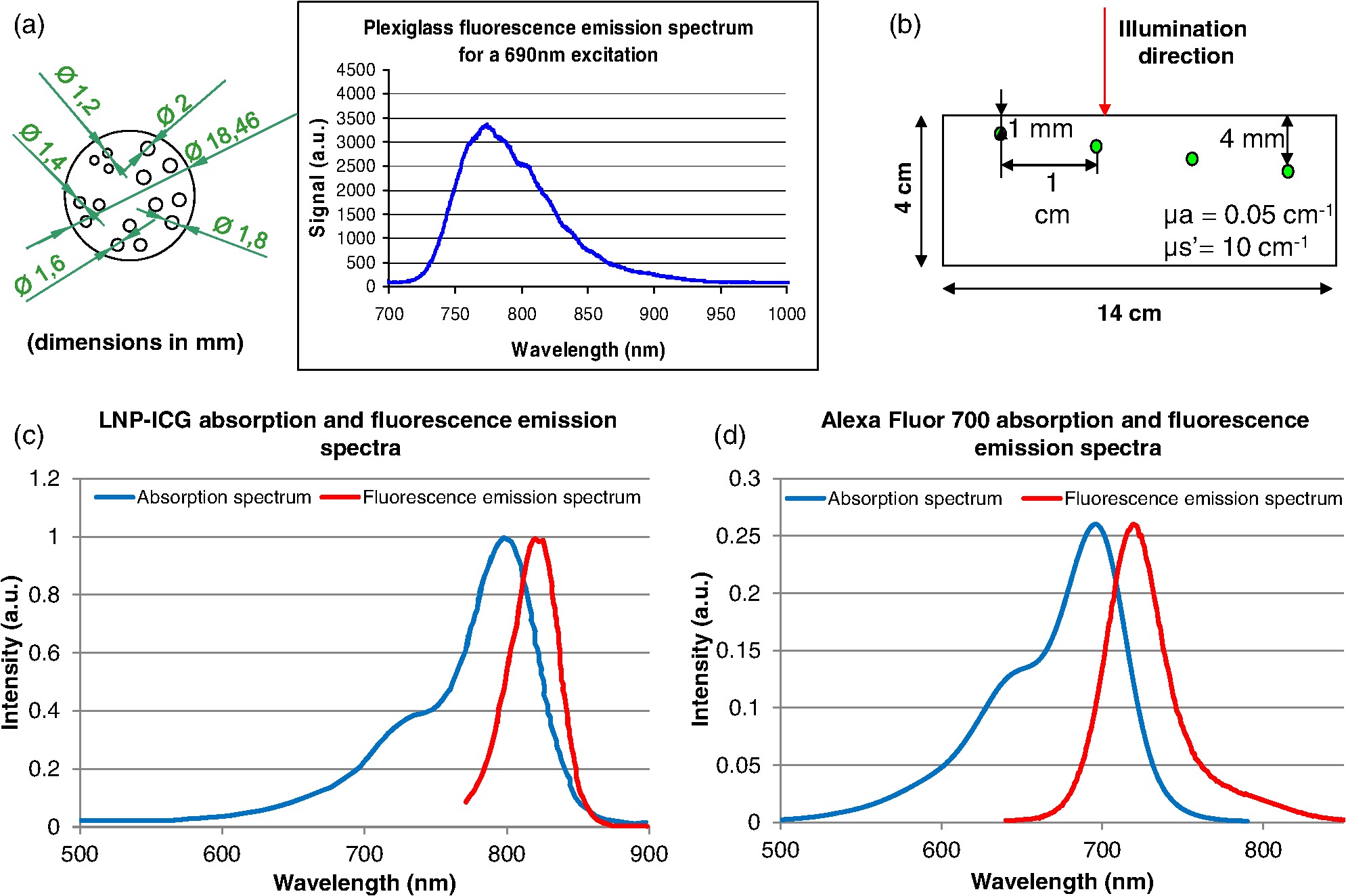 Three different types of phantoms were used for this study:
The in vivo validation of the method was performed with an adult female nude mouse. The animal procedure is in compliance with the guidelines of the European Union, taken in the French law regulating animal experimentation. All efforts were made to minimize the animal’s suffering. The mouse was anesthetized using a cocktail of ketamine and xylazine and was then placed on an adjustable platform with a warming pad. A capillary tube filled with of Alexa Fluor 700 at was inserted into the animal to simulate a marked target.31 The Alexa Fluor 700 absorption and fluorescence emission spectra are presented in Fig. 2(d). For this in vivo experiment, where Alexa Fluor 700 was used, we replaced the fluorescence filter with a RG9 700-nm long-pass Schott glass filter (ITOS) coupled with a 725/50-nm interference filter (Chroma Technology, Bellows Falls, Vermont). For this in vivo experiment, we also used translation steps to be able to use thinner detection stripes. Four hundred images were acquired for each depth considered with an integration time of 2 s. This leads to a total scanning time of 800 s. Again, no significant photobleaching was observed for any of the experiments. 2.2.Image Processing MethodsIn Fig. 3, we depict both LS-FRI methods and the way the equivalent of a classical wide-field FRI image is obtained (this equivalent will be referred to as WF-FRI and will be discussed in detail in the following section). We propose a schematic of three images from the acquired stack taken at different positions of the excitation line and the resulting images for WF-FRI and both LS-FRI methods. The difference between these methods is that, in one case (WF-FRI), all the information content of the images will be used by doing a sum of the stack, whereas in the other case (LS-FRI1), we will only detect one single stripe of pixels per image and concatenate all the detected stripes to obtain the whole field of view. In the last case (LS-FRI2), we also have another possibility; that of using the information contained in the adjacent stripes to get an insight of the background signal to subtract. In Fig. 3, the detected stripe is located directly over the excitation line and there is one given size for the neighboring area. We will see that both the location of the detection stripe and the size of the neighboring area can be optimized to improve the contrast. This will be explained in detail in the following subsections. Fig. 3Description of the image processing methods. (a) Schematic of images taken at three different positions of the excitation line. (b) Processing method for each detection scheme; : intensity in line of the image , : detection stripe (located over the excitation line in this example), : size of the neighboring area considered to calculate the background signal to subtract.  2.2.1.Wide-field image: WF-FRI/comparison with classical FRITo be able to qualitatively compare the LS-FRI methods to the classical FRI, we must first obtain the equivalent of a wide-field illumination image. As the illumination obtained with an expanded beam is the same as the one obtained from the sum of several illuminations covering the same area, we can obtain a WF-FRI image by summing the stack of images at all the positions with a shift depending on the translation step of the object (as depicted in the bottom left of Fig. 3). We compare Figs. 4(a) and 4(b) the images obtained with a real wide-field imaging system (FRI) and the sum of the stack of images (WF-FRI) when imaging the phantom with four inclusions. We can see that both images are similar (after taking into account the shape of the illumination for the real wide-field imaging system). The difference is that the signal-to-noise ratio is better with the sum of the images. This is explained by the fact that the integration time is virtually longer in the case of the sum of the stack of images. Smoothing the real wide-field image (with, for example, a median filter) would further increase the similarities between the two images, but the background noise would still be higher for the real wide-field illumination. Fig. 4Comparison between a real wide-field image (FRI) and the sum of the stack of images (WF-FRI) with the four inclusions phantom: (a) wide-field fluorescence image corrected with the excitation image to account for the shape of the illumination; (b) sum of the stack of images; (c) normalized intensity profiles for the real wide-field illumination (red dashed line) and the sum of the stack of images (blue solid line); images (a) and (b) are normalized, and the intensity profiles are taken perpendicularly to the capillaries along the black line traced on these images.  These observations can also be made when looking at the normalized intensity profiles plotted in Fig. 4(c). We see that both profiles overlap perfectly, the difference being that the real wide-field imaging profile is noisier than the one obtained with the sum of images. 2.2.2.Single stripe detection: LS-FRI1We will now present how the LS-FRI method takes the advantage of the stack of images for every position of the excitation line to enhance the contrast and resolution of the fluorescence signals. The first detection scheme that can be applied (referred to as LS-FRI1, depicted in Fig. 3) is to simply use the signal detected in a single stripe of pixel lines in each image rather than the whole image. We can then concatenate these detection stripes (depicted with red stripes in Fig. 3) to create the result image . To be able to have an image of the whole object studied without any gap or overlap, the detection stripe must have the right size in pixel lines which depends on the optical resolution of the system and on the size of the translation step between each image. To demonstrate how LS-FRI1 can improve the resolution compared with WF-FRI, we can use the diffusion equation. Its solutions with both illumination geometries are depicted in Fig. 5(a). Fig. 5(a) Geometries studied: planar for the wide-field illumination (top), cylindrical for line illumination (bottom); point and vector indicate the observation point, respectively, for the planar geometry and the cylindrical geometry; (b) geometry studied in simulation for the comparison of the resolutions in WF-FRI and LS-FRI1; (c) Full-widths at half maximum obtained when observing a single fluorescent inclusion located at different depths for LS-FRI1 (blue solid line) and WF-FRI (red dashed line). 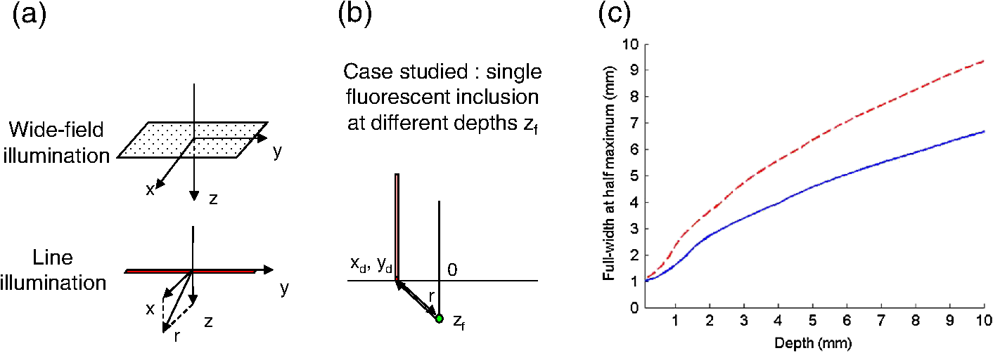 For a wide-field illumination in the steady-state regime in an infinite homogeneous medium, the diffusion equation solution is32 where is the fluence rate at point , is the source intensity, is the diffusion coefficient, and is the effective attenuation coefficient.For a line illumination, the solution is32 where is the modified Bessel function of the second kind of order 0.From these analytical solutions for a plane source and a line source, it is possible to simulate the improvement obtained with LS-FRI1. Let us have a look at the case of a single fluorescent inclusion at different depths in a medium with the optical properties of tissues [as depicted in Fig. 5(b)]. The fluorescence intensity calculations and from widefield and line illumination, respectively, derived from Eqs. (1) and (2) are calculated as follows: For the wide-field illumination, we have The conversion factor is equal to , where is the fluorophore extinction coefficient [], is the fluorophore concentration (), and is the fluorescence quantum yield which is dimensionless. For the diffusion coefficients and and the effective attenuation coefficients and , subscripts and denote, respectively, the excitation and fluorescence wavelengths. For a line illumination scanning the -axis with the detection on the excitation line, we have The variations of the full width at half maximum of the signal obtained with both formulas for depths ranging from 0.1 mm and 1 cm were calculated and are represented in Fig. 5(c). From this figure, we can clearly see that the resolution is better with LS-FRI1 compared with WF-FRI for all the depths addressed in this simulation. If the selected stripe is chosen directly on the excitation line, we can then compare this detection method to a confocal detection scheme with a virtual slit implemented in postprocessing. However, the selected stripe can also be chosen away from the excitation line. By selecting further stripes, we are able to probe deeper into the tissue as we take into account photons which were more scattered inside the medium. Using this method of detection decreases the overall amount of photons considered to obtain the result image. This way, the lateral resolution and the signal-to-background ratio can be improved as we do not sum the contributions of scattered photons from the fluorescence signal of interest and from parasite signals. 2.2.3.Single stripe detection with neighborhood subtraction: LS-FRI2Another possible detection scheme (referred to as LS-FRI2, depicted in the bottom right of Fig. 3) is to select a single stripe in as previously described and to subtract the mean intensity recorded in its neighboring areas of size (in pixels). The signal detected in the adjacent stripes is used as an estimate of the unwanted background signal and is subtracted from the central detected stripe. This detection scheme enhances the contrast mainly for the fluorescent objects close to the surface. The size considered for the areas can be the same as the detected stripe or it can be larger. We will see in Sec. 3 that the optimal size to use depends on the depth of the inclusion observed. 3.Results and DiscussionWe will present in this section the results obtained on optical phantoms in terms of contrast and resolution enhancements. We will then show preliminary in vivo results validating the interest of the proposed method in a realistic case. 3.1.Results on Optical PhantomsAll the results presented in this section have been obtained for a realistic fluorescence to background fluorescence ratio. This level of background fluorescence has been chosen using Ref. 33. We have used a concentrations’ ratio of about 80 between the fluorescent inclusion and the background medium (this is based on the “ICG equivalent” signal of skin which is the median one compared with the different organs, as presented in Ref. 33). 3.1.1.Contrast enhancementTo compare the different detection schemes (WF-FRI, LS-FRI1, and LS-FRI2) and to quantify the improvements, we introduce the contrast defined as where ; and ; are, respectively, the mean intensity values in a target region of interest (with fluorescence) and in a neutral region of interest (with background fluorescence only).The regions of interest were the same for the three techniques studied. The neutral region of interest was chosen in the top edge of the images so that it was the farthest possible from the target region of interest, while still being illuminated the same way, to ensure that the inhomogeneities of the illumination could not bias the results. The first set of results was obtained for a single fluorescent inclusion at different depths in a tissue-like liquid phantom, and the concentration of background fluorescence was set to have a realistic fluorescence to background ratio. We will first show a comparison between WF-FRI and both LS-FRI methods before and after optimizing their parameters, which are the excitation-detection distance for LS-FRI1 and the size of the neighboring area for LS-FRI2. After that, we will show the influence of these parameters on the contrast and how we chose them to optimize the results and get the best possible contrast for each depth. We plot in Fig. 6(a) the contrasts obtained with the three methods versus the depth of the inclusion when using basic parameters for both LS-FRI techniques [meaning that we do the detection directly on the excitation line () for LS-FRI1 and that the size of the neighboring area is equal to the size of the detection stripe () for LS-FRI2]. Fig. 6Comparison of the contrast obtained for a single fluorescent inclusion at 10 depths with the different methods with (a) basic parameters and (b) optimized parameters: WF-FRI (blue circles), LS-FRI1 (red squares), and LS-FRI2 (green x).  We can first notice that the LS-FRI1 (boxes) method increases the contrast compared with the WF-FRI (circles) for all depths addressed: there is a gain of about 1.4 when the inclusion is 1-mm deep and a gain of about 1.8 when the inclusion is 10-mm deep. With LS-FRI2 (crosses), the contrast observed is better than WF-FRI and comparable with LS-FRI1 when the inclusion is 1-mm deep, but after that it decreases and becomes worse than the one obtained with WF-FRI from 4 mm and deeper. This decrease is due to the overestimation of the parasite fluorescence when using an adjacent area size of 1 mm for inclusions which are not close enough to the surface. The results obtained with the different methods with optimized parameters (meaning the best excitation-detection distance for LS-FRI1 and the best neighboring area size for LS-FRI2) for all depths addressed in this experiment are summed up on Fig. 6(b). We see that both methods considered lead to an enhancement of the contrast when using the appropriate parameter. Choosing an optimized parameter is important mainly for LS-FRI2: for example, for an inclusion 10-mm deep, the contrast increases fivefold when choosing the right adjacent area size . The gain observed when using the optimized distance for LS-FRI1 is less important. To choose the method to obtain the best results depends on the depth of the fluorescent inclusion: for inclusions close to the surface, the LS-FRI2 offers a slightly better performance, but the LS-FRI1 is slightly better for the largest depths. We will now see how we obtained these improved results by using different parameters and for both LS-FRI techniques. We will show how and influence the contrast improvement for the different depths addressed. The results obtained when varying the LS-FRI1 parameter (which is the distance between the detection stripe and the excitation line) are presented in Fig. 7(a). The LS-FRI1 contrast results are plotted as a function of this parameter ( corresponds to detection over the excitation line and corresponds to detection at 10 mm away from the excitation line). The contrasts are normalized with the WF-FRI contrasts. Fig. 7Contrast obtained with (a) LS-FRI1 versus excitation-detection distance and (b) LS-FRI2 versus adjacent area size for one fluorescent inclusion located at: 1 mm (dark blue circles), 2 mm (pink stars), 3 mm (light green x), 4 mm (solid black), 5 mm (yellow +), 6 mm (red squares), 7 mm (light blue diamonds), 8 mm (violet down triangle), 9 mm (blue triangle), and 10 mm (brown side triangle).  As stated in the previous paragraph, we see that the contrast is increased for all the depths addressed if we do the detection over the excitation line, with gains varying between 1.4 and 1.8. But we also see on this graph that it is possible to have an even higher gain by choosing the appropriate excitation-detection distance . Furthermore, this optimal distance seems to be related to the depth of the inclusion observed: the deeper the inclusion, the larger the distance for the best contrast. For example, the best contrast is achieved for a detection over the excitation when the inclusion is 1-mm deep, but the maximum contrast is obtained for a detection 4 mm away from the excitation line when looking at an inclusion 10-mm deep. Figure 7(b) shows the results obtained when varying the LS-FRI2 parameter (which is the size of the neighboring area used to have an estimate of the parasite signal). Twenty sizes of areas ranging from 1 to 20 mm were considered for the calculation of the signal to subtract. The LS-FRI2 contrast results are plotted here as a function of the size of the adjacent area (in millimeters). The contrasts are also normalized with the WF-FRI contrasts. As previously mentioned, we see that the gain is only superior to 1 for the first 4 mm when using a 1-mm surrounding area. Beyond this depth, the fluorescence signal of interest varies too slowly for the surrounding positions of excitation around the fluorescent inclusion. It is then necessary to use larger neighboring areas to calculate the signal to be subtracted to improve the contrast. Similar to the observation made for the variation of the LS-FRI1 parameter, there is a relationship between the optimal area size for the maximum gain and the depth of the inclusion: the deeper the inclusion, the larger the area to consider for the best contrast. For example, while the gain is nearly the same whether the adjacent area is 1-mm large or 20-mm large when the inclusion is 1-mm deep, it increases from about 0.3 for a 1-mm area to about 1.5 for a 20-mm area when the inclusion is 10-mm deep. 3.1.2.Resolution enhancementAfter these contrast studies, we will focus on the main objective, the resolution enhancement. To obtain this second set of results, we used the fluorescent resolution target described in the previous part [Fig. 2(a)]. The concentration of background fluorescence was set to have a realistic fluorescence to background ratio as in the previous experiment, and the target was submerged at four depths between 1 and 4 mm. Before doing this study, we will give information on the influence of the scanning direction, which can affect the resolution enhancement. On Fig. 8, we show the images obtained with LS-FRI1 and LS-FRI2 for two perpendicular scanning directions. For this example, the fluorescent target is located at 1-mm under the surface. Fig. 8Images of the fluorescent target at a depth of 1 mm obtained with the LS-FRI methods using two perpendicular scanning directions. 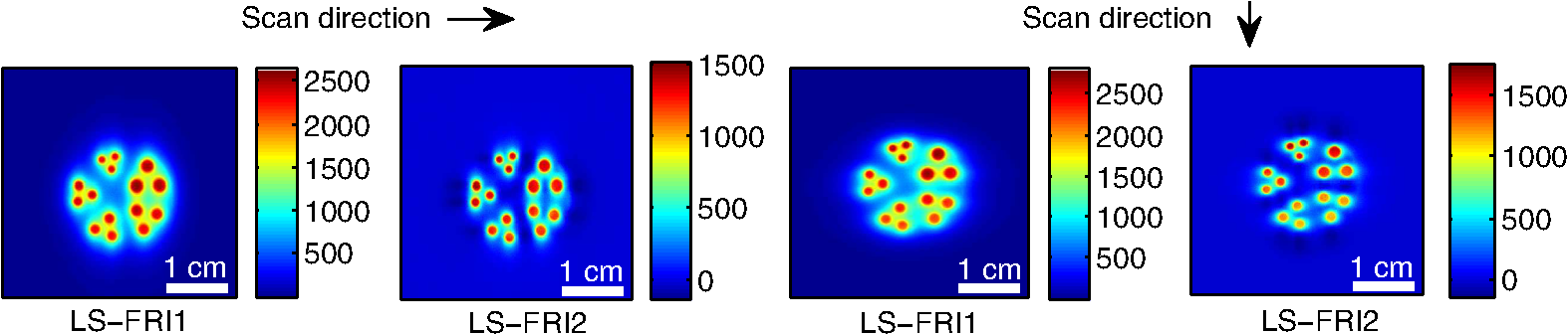 We clearly see on this figure that the scanning direction has an influence on the resolution improvement. If we look at the two images on the left, the resolution is mainly enhanced with LS-FRI methods in the same direction as the scanning direction as indicated by the arrow. This observation is the same for the perpendicular scanning direction depicted in the two images on the right. The images obtained with WF-FRI (not represented here) are the same in both scanning directions, as expected. For the results that we will now present, we used both scanning directions and did the sum of the two images obtained to have the most homogeneous resolution possible in the and directions. Furthermore, this sum compensates the scanning artifacts that appear with LS-FRI2 for small values of the parameter (these artifacts can be seen on Fig. 8). We give the resulting images for the three methods at the four depths considered in Fig. 9, and we focus on the improvement of the depth detection associated with the resolution enhancement. For this experiment, basic parameters were used for both LS-FRI techniques ( for LS-FRI1 and for LS-FRI2) to be closer to a real case where no depth information is available. Fig. 9Images of the fluorescent target at four different depths from 1 to 4 mm obtained with the three methods.  For WF-FRI (left column), it is possible to resolve the target only at 1 mm, but there is already some crosstalk between the different groups of inclusions, leading to an overestimation of the signal produced by the largest inclusions. At 2 mm, it is not possible to distinguish the five groups, the signals coming from the three largest groups of inclusions start to overlap and form one large fluorescent signal. At 3 mm, the whole target only emits one large fluorescent signal and the groups of inclusions are completely unresolved. At 4 mm, the large fluorescent signal becomes even more uniform, and the real shape of the target is completely undistinguishable. The LS-FRI1 (central column) is slightly better. It enhances the resolution as it increases the peak-to-valley ratio between the fluorescent inclusions and the background, but there is still a background signal surrounding the inclusions due to the scattering. At 1 mm, individual spots are visible in each group. At 2 mm, a detection can be done for the five groups but no individual spot is visible. At 3 mm, the performance decreases as only the two smallest groups of inclusions stay resolved, while the three largest ones emit overlapping signals. At 4 mm, the target is nearly completely unresolved as the different contributions due to scattering join to form a large fluorescence signal similar to the one obtained with WF-FRI at 3 mm. The LS-FRI2 (right column) offers the best performance as the background signal is well suppressed. At 1 mm, each individual spot is clearly visible in each group. At 2 mm, the resolution between the groups of inclusions is good and it is still possible to detect the single inclusions inside each group. At 3 mm, the method still allows a clear separation between the different groups of inclusions. We can also distinguish three inclusions in the two largest groups. At 4 mm, even if the single inclusions inside the different groups become unresolved, it is still possible to see five distinct groups of inclusions. These results obtained with the fluorescent resolution target are a good example of the advantage of our method compared with a simple image processing algorithm: because we only select certain photons with LS-FRI techniques, it would not be possible to obtain these results by applying a denoising image processing algorithm directly on the WF-FRI images. The third and last set of results was obtained with four fluorescent inclusions located at increasing depths [Fig. 2(b)]. The concentration of background fluorescence was set to have a realistic fluorescence to background ratio as in the previous experiments. We want to underline the fact that the illumination line was parallel to the inclusions for these results. As we saw with the previous results, the illumination direction has an influence on the resolution improvement, even more with these results where the fluorescent inclusions are cylindrical capillaries. In Figs. 10(a), 10(b), and 10(c), we see, respectively, the images obtained with WF-FRI, LS-FRI1, and LS-FRI2. These images show how the overall visibility is enhanced with LS-FRI methods: with WF-FRI, the four inclusions can be detected but the spatial resolution is low due to the large scattering of photons around the inclusions. The scattered fluorescence signal from the inclusions closest to the surface adds to the signal from the deepest inclusions, leading to misinterpretations. With the LS-FRI1, the spatial resolution of the four inclusions is improved. As with the resolution target, the best resolution can be obtained with the LS-FRI2 for the first two inclusions where it is possible to spatially describe the inclusions. Fig. 10(a) Image obtained with WF-FRI; (b) Image obtained with LS-FRI1; (c) Image obtained with LS-FRI2 (top view); (d) Normalized intensity profiles obtained with: WF-FRI (blue circles), LS-FRI1 (red squares), and LS-FRI2 (green x); images (a), (b), and (c) are normalized.  In this experiment, the parameters chosen for LS-FRI techniques were optimized for the capillaries closest to the surface ( for LS-FRI1 and for LS-FRI2). This shows the tradeoff of the technique in a case where several depths are addressed at the same time: the signal coming from the two deepest inclusions is very weak, making them almost invisible. Intensity profiles presented on Fig. 10(d) show the improvements of LS-FRI techniques over WF-FRI. 3.2.In Vivo ValidationAfter these phantom experiments to prove the contrast and resolution enhancements, we will validate the LS-FRI methods on an in vivo situation. For the in vivo validation, we decided to study a challenging case where classical FRI systems reach their limits. We inserted in the mouse a capillary filled with of Alexa Fluor 700 at as previously described to simulate a fluorescent target in the thorax region at a depth of about 6 mm. Because of the optical heterogeneity of the area and the depth of the inclusion, classical planar FRI systems can have difficulties in obtaining a good signal-to-background ratio.34 Similar to the resolution enhancement results on liquid phantoms, two scanning directions (sagittal and transverse) were used and their results were summed to avoid the scanning artifacts. In Fig. 11(a), we first present a white light image with the capillary outside the mouse to give an idea of the transverse localization of the fluorescence. Figures 11(b) and 11(c) show the WF-FRI images with and without the capillary filled with Alexa Fluor 700. Even if there is a fluorescence signal present [Fig. 11(b)], it is lost within the background signal of the mouse. This background signal originates from a sum of the autofluorescence of the mouse and of some of the excitation signal that was not completely filtered. The general high intensity of this background signal is due to the relatively long integration time (2 s) used to acquire each of the 400 images used in this experiment. Fig. 11(a) White light image with the capillary outside the mouse to show the localization of the fluorescence of interest. (b) WF-FRI image with the capillary inserted. (c) Control experiment: WF-FRI image without the capillary inserted. (d) LS-FRI1 image with the capillary inserted obtained with an 8-mm excitation-detection distance. (e) LS-FRI1 image without the capillary inserted obtained with an 8-mm excitation-detection distance. 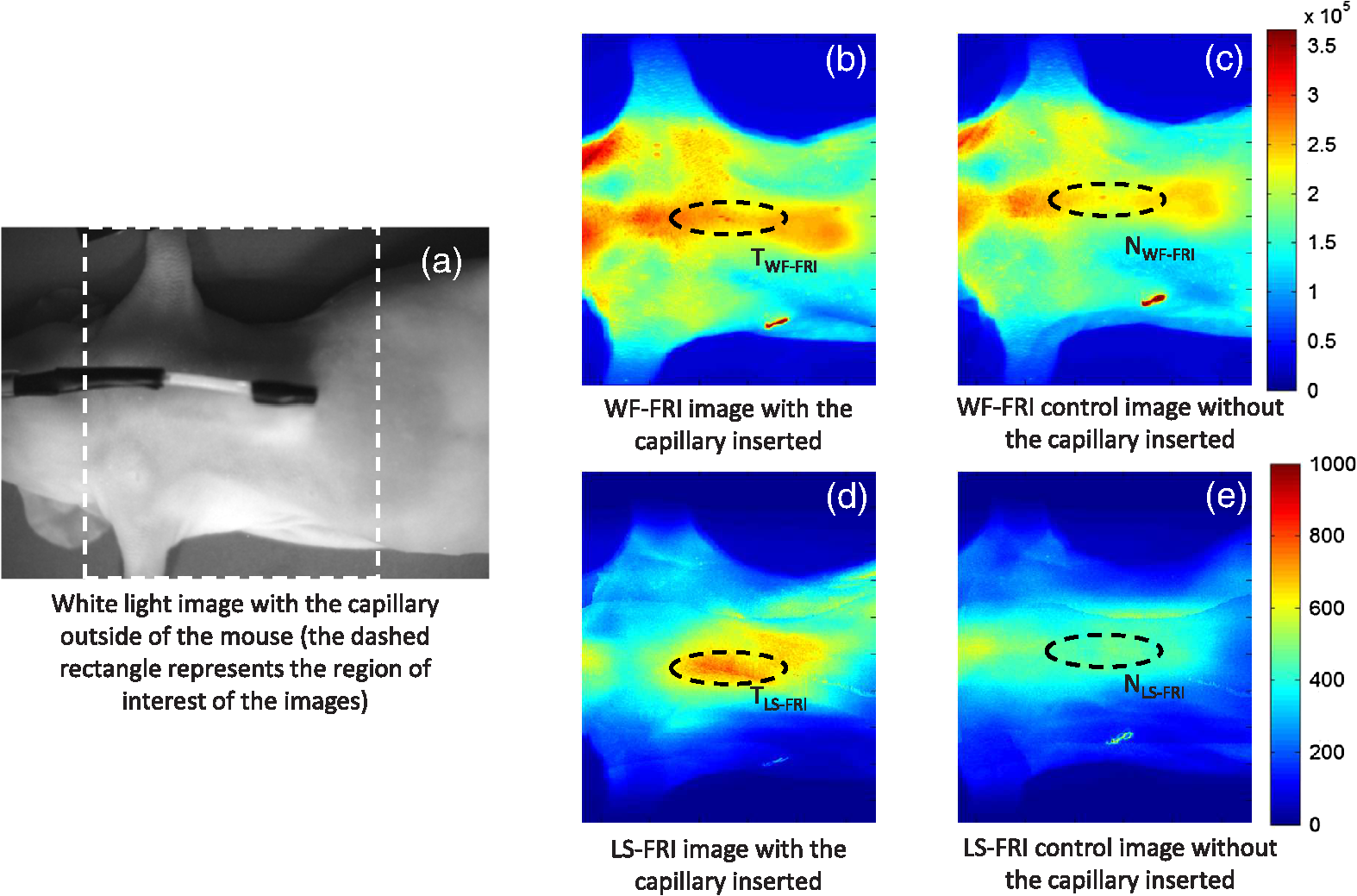 We can see on the control image [Fig. 11(c)] that there is a comparable fluorescence signal although there is no capillary. The contrast obtained when using the regions of interest and depicted in the figures is about 0.07. This shows that a classical FRI device would not be usable in this particular case. Because of the depth of the capillary and the weak fluorescence to background fluorescence ratio, LS-FRI1 was better suited than LS-FRI2 to improve the WF-FRI results. In order to choose the best imaging protocol, we applied the LS-FRI1 method with different excitation-detection distances . We studied 10 different distances ranging from 1 to 10 mm and observed the best results with a distance of . To achieve a field of view comparable with the WF-FRI one, we summed the LS-FRI images obtained with excitation-detection distances in both directions. Figures 11(d) and 11(e) show the LS-FRI1 images for an excitation-detection distance of 8 mm with and without the capillary filled with Alexa Fluor 700. We see that the LS-FRI1 is able to detect a fluorescence signal located where the capillary should be [Fig. 11(d)], while this signal is not present in the corresponding control image [Fig. 11(e)]. The contrast obtained when using the regions of interest and depicted in the figures is about 0.24, which is more than three times better than the one obtained with the classical WF-FRI. The real advantage of the method is the suppression of a large amount of parasite fluorescence which allows a clearer detection of the fluorescence of interest. Due to the geometry of our setup, the shape of the laser line was deformed by the body contour of the mouse. This implied a more complex postprocessing of the images to get the real shape of the laser line to be able to correctly implement LS-FRI methods. Yet, performing the detection on a straight line as in the previous experiments could still enhance the results obtained compared with WF-FRI. Furthermore, we are currently working on the optical setup to find the best compromise concerning the excitation so that LS-FRI could be implemented in real time without being impacted by the shape of the object studied. 4.ConclusionWe presented in this paper a novel approach for molecular imaging based on the use of a laser line illumination rather than the classical wide-field FRI. By using a laser line to illuminate the object to study and acquiring images for each position of the line, we have access to a large amount of information that we can use with different image processing methods. We proved that these techniques allow us to enhance the contrast and resolution of fluorescent targets and reduce the effect of parasite signals such as background fluorescence on phantoms mimicking tissue-like optical properties. The methods were also tested in vivo in the case of a fluorescent source in the thorax region, where imaging the fluorescence usually proves to be difficult. We were able to notably improve the results and to overpass the classical WF-FRI scheme, which is unable to detect a usable signal in this optically heterogeneous area. As we have seen with the contrast enhancement results, the quality of the images is affected by the choice of the and parameters of LS-FRI techniques. Still, the resolution enhancement results obtained with the fluorescent target show that even without using optimized parameters, LS-FRI techniques offer better performance than WF-FRI. Furthermore, the relationship between the LS-FRI parameters and the depth of fluorescence signal could also be used in 3-D reconstruction approaches. While all the results presented here have been obtained by postprocessing the images to be able to do a proof of principle, we are currently working on the limiting factors of the method (such as the effect of the scanning direction and the influence of the surface of the object on the line shape) to be able to apply it in real time. Furthermore, a specific optical setup is envisioned to offer the opportunity to implement LS-FRI methods. The target setup is based on the bilateral scanning confocal microscope from Brakenhoff and Visscher,35 but with a programmable mask in the imaging plane in place of the confocal setup detector pinhole so as to select the stripes to detect in real time. By choosing an appropriate integration time for the camera and synchronizing it with the scanning system, we would be able to acquire an image of the whole field targeted on the object and directly perform the previously presented methods. AcknowledgmentsThe authors would like to thank Dr. Véronique Josserand (INSERM-UJF U823) and the “OPTIMAL small animal optical imaging facility” for their support for the in vivo study. ReferencesJ. V. Frangioni,
“In vivo near-infrared fluorescence imaging,”
Current Opin. Chem. Biol., 7
(5), 626
–634
(2003). http://dx.doi.org/10.1016/j.cbpa.2003.08.007 COCBF4 1367-5931 Google Scholar
V. NtziachristosC. BremerR. Weissleder,
“Fluorescence imaging with near-infrared light: new technological advances that enable in vivo molecular imaging,”
Eur. Radiol., 13
(1), 195
–208
(2003). EURAE3 1432-1084 Google Scholar
E. M. Sevick-MuracaJ. P. HoustonM. Gurfinkel,
“Fluorescence-enhanced, near infrared diagnostic imaging with contrast agents,”
Curr. Opin. Chem. Biol., 6
(5), 642
–650
(2002). http://dx.doi.org/10.1016/S1367-5931(02)00356-3 COCBF4 1367-5931 Google Scholar
S. A. HilderbrandR. Weissleder,
“Near-infrared fluorescence: application to in vivo molecular imaging,”
Curr. Opin. Chem. Biol., 14
(1), 71
–79
(2010). http://dx.doi.org/10.1016/j.cbpa.2009.09.029 COCBF4 1367-5931 Google Scholar
R. Y. Tsien,
“Building and breeding molecules to spy on cells and tumors,”
FEBS Lett., 579
(4), 927
–932
(2005). http://dx.doi.org/10.1016/j.febslet.2004.11.025 FEBLAL 0014-5793 Google Scholar
M. FunovicsR. WeisslederC.-H. Tung,
“Protease sensors for bioimaging,”
Anal. Bioanal. Chem., 377
(6), 956
–963
(2003). http://dx.doi.org/10.1007/s00216-003-2199-0 ABCNBP 1618-2642 Google Scholar
R. Weisslederet al.,
“In vivo imaging of tumors with protease-activated near-infrared fluorescent probes,”
Nat. Biotechnol., 17
(4), 375
–378
(1999). http://dx.doi.org/10.1038/7933 NABIF9 1087-0156 Google Scholar
S. L. Troyanet al.,
“The FLARE intraoperative near-infrared fluorescence imaging system: a first-in-human clinical trial in breast cancer sentinel lymph node mapping,”
Ann. Surg. Oncol., 16
(10), 2943
–2952
(2009). http://dx.doi.org/10.1245/s10434-009-0594-2 1068-9265 Google Scholar
S. Giouxet al.,
“FluoSTIC: miniaturized fluorescence image-guided surgery system,”
J. Biomed. Opt., 17
(10), 106014
(2012). http://dx.doi.org/10.1117/1.JBO.17.10.106014 JBOPFO 1083-3668 Google Scholar
C. Hircheet al.,
“An experimental study to evaluate the fluobeam 800 imaging system for fluorescence-guided lymphatic imaging and sentinel node biopsy,”
Surg. Innovation, 20
(5), 516
–523
(2013). http://dx.doi.org/10.1177/1553350612468962 1553-3506 Google Scholar
J. Hunget al.,
“Autofluorescence of normal and malignant bronchial tissue,”
Lasers Surg. Med., 11
(2), 99
–105
(1991). http://dx.doi.org/10.1002/(ISSN)1096-9101 LSMEDI 0196-8092 Google Scholar
S. GiouxH. S. ChoiJ. V. Frangioni,
“Image-guided surgery using invisible near-infrared light: fundamentals of clinical translation,”
Mol. Imaging, 9
(5), 237
–255
(2010). MIOMBP 1535-3508 Google Scholar
S. BhaumikJ. DePuyJ. Klimash,
“Strategies to minimize background autofluorescence in live mice during noninvasive fluorescence optical imaging,”
Lab Anim., 36
(8), 40
–43
(2007). http://dx.doi.org/10.1038/laban0907-40 LBANAX 0023-6772 Google Scholar
Y. Inoueet al.,
“Diet and abdominal autofluorescence detected by in vivo fluorescence imaging of living mice,”
Mol. Imaging, 7
(1), 21
–27
(2008). MIOMBP 1535-3508 Google Scholar
S. MacLaurinet al.,
“Reduction of skin and food autofluorescence in different mouse strains through diet changes,”
(2006). Google Scholar
V. Chernomordiket al.,
“Inverse method 3-d reconstruction of localized in vivo fluorescence-application to sjogren syndrome,”
IEEE J. Sel. Top. Quantum Electron., 5
(4), 930
–935
(1999). http://dx.doi.org/10.1109/2944.796313 IJSQEN 1077-260X Google Scholar
A. Eidsathet al.,
“Three-dimensional localization of fluorescent masses deeply embedded in tissue,”
Phys. Med. Biol., 47
(22), 4079
–4092
(2002). http://dx.doi.org/10.1088/0031-9155/47/22/311 PHMBA7 0031-9155 Google Scholar
C. D'Andreaet al.,
“Localization and quantification of fluorescent inclusions embedded in a turbid medium,”
Phys. Med. Biol., 50
(10), 2313
–2327
(2005). http://dx.doi.org/10.1088/0031-9155/50/10/009 PHMBA7 0031-9155 Google Scholar
V. NtziachristosR. Weissleder,
“Experimental three-dimensional fluorescence reconstruction of diffuse media by use of a normalized Born approximation,”
Opt. Lett., 26
(12), 893
–895
(2001). http://dx.doi.org/10.1364/OL.26.000893 OPLEDP 0146-9592 Google Scholar
A. SoubretV. Ntziachristos,
“Fluorescence molecular tomography in the presence of background fluorescence,”
Phys. Med. Biol., 51
(16), 3983
–4001
(2006). http://dx.doi.org/10.1088/0031-9155/51/16/007 PHMBA7 0031-9155 Google Scholar
V. Ntziachristoset al.,
“Fluorescence molecular tomography resolves protease activity in vivo,”
Nat. Med., 8
(7), 757
–760
(2002). http://dx.doi.org/10.1038/nm729 1078-8956 Google Scholar
A. Joshiet al.,
“Molecular tomographic imaging of lymph nodes with NIR fluorescence,”
in 4th IEEE Int. Symposium on Biomedical Imaging: From Nano to Macro, 2007. ISBI 2007,
564
–567
(2007). Google Scholar
M. A. A. NeilR. JuskaitisT. Wilson,
“Method of obtaining optical sectioning by using structured light in a conventional microscope,”
Opt. Lett., 22
(24), 1905
–1907
(1997). http://dx.doi.org/10.1364/OL.22.001905 OPLEDP 0146-9592 Google Scholar
M. G. L. Gustafsson,
“Nonlinear structured-illumination microscopy: wide-field fluorescence imaging with theoretically unlimited resolution,”
Proc. Natl. Acad. Sci. U. S. A., 102
(37), 13081
–13086
(2005). http://dx.doi.org/10.1073/pnas.0406877102 PNASA6 0027-8424 Google Scholar
F. ChaslesB. DubertretA. C. Boccara,
“Optimization and characterization of a structured illumination microscope,”
Opt. Express, 15
(24), 16130
–16140
(2007). http://dx.doi.org/10.1364/OE.15.016130 OPEXFF 1094-4087 Google Scholar
E. Mudryet al.,
“Structured illumination microscopy using unknown speckle patterns,”
Nat. Photonics, 6
(5), 312
–315
(2012). http://dx.doi.org/10.1038/nphoton.2012.83 1749-4885 Google Scholar
A. J. Linet al.,
“Spatial frequency domain imaging of intrinsic optical property contrast in a mouse model of Alzheimers disease,”
Ann. Biomed. Eng., 39
(4), 1349
–1357
(2011). http://dx.doi.org/10.1007/s10439-011-0269-6 ABMECF 0090-6964 Google Scholar
A. Mazharet al.,
“Structured illumination enhances resolution and contrast in thick tissue fluorescence imaging,”
J. Biomed. Opt., 15
(1), 010506
(2010). http://dx.doi.org/10.1117/1.3299321 JBOPFO 1083-3668 Google Scholar
S. D. Koneckyet al.,
“Quantitative optical tomography of sub-surface heterogeneities using spatially modulated structured light,”
Opt. Express, 17
(17), 14780
–14790
(2009). http://dx.doi.org/10.1364/OE.17.014780 OPEXFF 1094-4087 Google Scholar
F. P. Navarroet al.,
“A novel indocyanine green nanoparticle probe for non invasive fluorescence imaging in vivo,”
Proc. SPIE, 7190 71900L
(2009). http://dx.doi.org/10.1117/12.808195 PSISDG 0277-786X Google Scholar
J. Boutetet al.,
“Optical tomograph optimized for tumor detection inside highly absorbent organs,”
Opt. Eng., 50
(5), 053203
(2011). http://dx.doi.org/10.1117/1.3574768 OPEGAR 0091-3286 Google Scholar
S. L. Jacques,
“Light distributions from point, line and plane sources for photochemical reactions and fluorescence in turbid biological tissues,”
Photochem. Photobiol., 67
(1), 23
–32
(1998). http://dx.doi.org/10.1111/php.1998.67.issue-1 PHCBAP 0031-8655 Google Scholar
A. M. De Grandet al.,
“Tissue-like phantoms for near-infrared fluorescence imaging system assessment and the training of surgeons,”
J. Biomed. Opt., 11
(1), 014007
(2006). http://dx.doi.org/10.1117/1.2170579 JBOPFO 1083-3668 Google Scholar
C. A. DiMarzioM. Niedre,
“Pre-clinical optical molecular imaging in the lung: technological challenges and future prospects,”
J. Thorac. Dis., 4
(6), 556
–557
(2012). JTDOBK 2072-1439 Google Scholar
G. J. BrakenhoffK. Visscher,
“Confocal imaging with bilateral scanning and array detectors,”
J. Microsc., 165
(1), 139
–146
(1992). http://dx.doi.org/10.1111/jmi.1992.165.issue-1 JMICAR 0022-2720 Google Scholar
|


