Full time-resolved diffuse fluorescence tomography accelerated with parallelized Fourier-series truncated diffusion approximation

Xi Yi; Bingyuan Wang; Wenbo Wan; Yihan Wang; Yanqi Zhang; Huijuan Zhao; Feng Gao

doi:10.1117/1.JBO.20.5.056003

12 May 2015 Full time-resolved diffuse fluorescence tomography accelerated with parallelized Fourier-series truncated diffusion approximation

Xi Yi, Bingyuan Wang, Wenbo Wan, Yihan Wang, Yanqi Zhang, Huijuan Zhao, Feng Gao

Author Affiliations +

Journal of Biomedical Optics, Vol. 20, Issue 5, 056003 (May 2015). https://doi.org/10.1117/1.JBO.20.5.056003

Abstract

Of the three measurement schemes established for diffuse fluorescence tomography (DFT), the time-domain scheme is well known to provide the richest information about the distribution of the targeting fluorophore in living tissues. However, the explicit use of the full time-resolved data usually leads to a considerably lengthy time for image reconstruction, limiting its applications to three-dimensional or small-volume imaging. To cope with the adversity, we propose herein a computationally efficient scheme for DFT image reconstruction where the time-dependent photon density is expanded to a Fourier-series and calculated by solving the independent frequency-domain diffusion equations at multiple sampling frequencies with the support of a combined multicore CPU-based coarse-grain and multithread GPU-based fine-grain parallelization strategy. With such a parallelized Fourier-series truncated diffusion approximation, both the time- and frequency-domain inversion procedures are developed and validated for their effectiveness and accuracy using simulative and phantom experiments. The results show that the proposed method can generate reconstructions comparable to the explicit time-domain scheme, with significantly reduced computational time.

1. Introduction

Diffuse fluorescent tomography (DFT) is being increasingly used as a noninvasive and highly sensitive method to image the fluorescent properties of tissues that report physiopathological processes in intact organisms, preferably using near-infrared radiation.¹^–⁴ And its methodology has been extensively explored within the framework of three measurement techniques in diffuse optics.⁵^,⁶ In comparison with the continuous-wave (CW) and frequency-domain (FD) modes, the time-domain (TD) approach acquires much richer information about the fluorophore distribution in a living tissue and, therefore, offers potential to achieve higher spatial resolution, better recovered contrast, as well as effective separation among multiple properties (yield and lifetime) and compositions.⁷^–¹⁰ Gao et al. have developed a finite-element time-difference photon diffusion modeling to solve the time-dependent coupled diffusion equations. Results show that the TD–DFT simultaneous reconstruction of the fluorescent yield and lifetime in a two-dimensional (2-D) circular domain can achieve superior quantitative accuracy, spatial resolution, and noise robustness, than using CW or transformed FD reconstructions.¹¹ Zhu et al. have also applied finite element based TD–DFT model to a three-dimensional (3-D) mouse model. Simulative results demonstrate that the incorporation of early and late time-bins can effectively improve the image accuracy.¹² However, since the photon migration modeling, i.e., the forward calculation, normally requires adequate recursive steps to temporally resolve the relevant physical quantities (boundary flux and interior photon density) at a numerically stable interval, the conventional approach of TD–DFT image reconstruction that explicitly uses the full time-resolved (TR) data with no parallelization potentials usually leads to a lengthy computational process, especially for 3-D scenarios and large-sized tissues, such as those in small animal whole-body imaging or optical mammography.¹³^–¹⁶

Until now, many approaches have been proposed to reduce the computational complexity of the TD–DFT problems.¹⁷^–²⁰ Holt et al. have proven that proper multiple time gates are important to provide superior image accuracy in TD–DFT when compared to the CW-DFT method.¹⁷ Furthermore, an overlap time gate is applied by Li to achieve better spatial resolution and fidelity, compared to those using the CW mode and traditional multiple time gate.²¹ Most of the aforementioned approaches are based on a featured-data scheme utilizing either Mellin or Laplace transformation of the time-dependent diffusion model, which has been proven to be computationally simple and demonstrate redundancy reduction.¹⁹^,²⁰ However, since the high-order Mellin or real-number Laplace transformation is prone to be highly correlated, increasingly subjected to noise, and/or mathematically incomplete, simulative and experimental reconstructions with such a scheme both exhibit inferior quantitative performance and poor spatial resolution than directly using the full time-resolved measurements, severely limiting its application in high-fidelity imaging. Therefore, to uncover the potential of TD–DFT for clinically required accuracy and spatial details in an effective way, there is a critical need to effectively use the full profiles of the TR measurements.

Since the TD system is mathematically equivalent to the combination of many FD ones employing a wide range of modulation frequencies, a Fourier transformation can therefore be used to possess the approximate optical information about the fluorophore distribution in a TD measurement mode. Recently, Pulkkinen et al. have employed a truncated Fourier-series approximation to simplify the finite-element solutions of the TD radiative transfer equation. Simulations on a homogeneous rectangular computational domain show that although the method with truncated Fourier-series approximation requires more memory and time to solve the equation of a singular frequency component, than that with the time-difference solution of a single temporal step, the total time of the former with 35 frequency components is only 1/5th that of the latter with 400 temporal steps, which greatly shortens the calculation time.²² However, the studies are only for the forward calculations of a 2-D domain. Ziegler et al. have applied the Fourier transformation to the nonlinear DFT reconstruction of a 3-D compressed breast-simulating phantom in a transmission-reflection measurement pattern, where the nearest source–detector distance is 10 mm, and only three angular frequency components are needed to obtain an accurate TR data.²³ However, the number is severely insufficient for applications with a smaller source–detector distance or larger size, where quite a number of frequency components and a long computation time are required. On that occasion, it is more significant to expand the truncated Fourier-series strategy to the full TR-DFT reconstruction problem, where a great challenge lies in the computational efficiency and severely increased unsuitability of obtaining the accurate anatomical structure and pathological information, due to the rapid growing in the number of the unknowns and the nonlinear dependency of the measurements on the optical properties. Conveniently, a parallelization strategy is necessary and easily utilized in the reconstruction.

To better take advantages of the TR measurements while effectively reducing the lengthy computation time incurred from the requisite temporal steps, we herein propose a parallelized Fourier-series truncated diffusion approximation (DA) to accelerate the full TR-DFT reconstruction. In our scheme, the time-dependent photon density is expanded to a Fourier series, based on which the TD diffusion equation (DE) can be solved through a series of independent FD–DEs at multiple sampling frequencies. Moreover, a combined multicore CPU-based coarse-grain and multithread GPU-based fine-grain parallelization strategy is employed to accelerate the process. The resulting temporal point spread functions (TPSFs) are tested in comparison with those of TD finite-difference (TDFD) solution and Monte Carlo (MC) simulation. With such forward calculations, both the TD and FD inversion procedures are developed based on a block algebraic reconstruction technique (ART). Simulations and phantom experiments are performed to compare with the explicit TD scheme to validate the accuracy and computational resources of the proposed method.

2. Methods

In general, the goal of DFT reconstruction (referred to as the inverse problem) is to quantitatively derive the distributions of the fluorescent properties in a tissue domain, by fitting the model predictions (referred to as the forward problem) to the diffusive excitation and emission light measurements on the boundary.

2.1.

Fourier-Series Truncated DE for Full TR Data

For the TD forward problem, the model-predicted boundary flux is calculated using the Fick’s law with the Robin boundary condition, under the Galerkin finite-element method (FEM) to transform the continuous DE into an $N$ -dimensional discrete problem of finding the nodal field photon density $Φ (r_{i}, t)$ at all nodes $r_{i} (i = 1,2, \dots, N)$ ; the resulting matrix equation can be given by²⁴

Eq. (1)

{\begin{cases} [K (κ_{ν}) + C (μ_{a ν} c)] Φ_{ν} (t) + B \frac{\partial Φ_{ν} (t)}{\partial t} = Q_{ν} (t) - b_{ν} (t) \\ Γ_{ν} (t) = \frac{c}{2} \frac{1 - R_{f}}{1 + R_{f}} Φ_{ν} (t) \end{cases},

where

K, C, B \in R^{N \times N}

are symmetric sparse matrices.

Φ

is the photon density under the source

Q

and the boundary quantity

b

.

Γ

is the measured boundary flux. The subscript

ν = [x, m]

denotes the variation at the excitation or the emission wavelength, respectively,

κ = {[3 (μ_{a} + μ_{s}^{'})]}^{- 1}

is the diffusion coefficient with an absorption coefficient

μ_{a}

and a reduced scattering coefficient

μ_{s}^{'}

.

c

denotes the speed of light in the medium and

R_{f}

is the internal reflection coefficient on the boundary.

To reduce the amount of the full TR data that is too large to be handled on the hardware within an acceptable period, one can either use the temporal filters or carry out the calculation in the FD. In our approach, we choose the second strategy by approximating the TD photon density $Φ (r, t)$ as a weighted combination of the truncated Fourier series at multiple frequency components:

Eq. (2)

Φ (r, t) = \sum_{k = - N_{ω}}^{N_{ω}} Φ (r, ω_{k}) \exp (j ω_{k} t),

where

Φ (r, ω_{k})

denotes the frequency component with Fourier frequency

ω_{k} (k = 0,1, \dots, N_{ω})

, whose choice is shown in Sec. 2.3.

Thus, the TD forward calculation can be obtained by solving a series of uncorrelated FD–DEs.

Eq. (3)

[K (κ_{ν}) + C (μ_{a ν} c) + j ω {}_{k}B] Φ_{ν} (ω_{k}) = Q_{ν} (ω_{k}) - b_{ν} (ω_{k}), k = 0,1, \dots, N_{ω} .

2.2.

Full TR–DFT Method with Fourier-Series Truncated DE

Before directly using the TR measurement for the image reconstruction, several necessary data preprocessing steps are acquired. First, as only a finite interval of the collected TPSF data is of interest, an identical start–end time is chosen to cover the most effective range of the TPSF curve, for an efficient implementation of the subsequent Fourier transformation. Second, to reduce the amount of calculation and effectively enhance the noise robustness of the reconstructions while still preserving the advantages of the full TR scheme, an overlap-delaying time gate method is employed to deal with the measurements.²¹ Third, a self-normalized data type as described in Ref. 11 is employed in the research to avoid the required scaling-factor calibration and spectroscopic characterization of the experimental system, and effectively reduce the adversity of system fluctuations that may occur between excitation and emission measurements.

To simplify the validation of the proposed method, we only consider the reconstruction of fluorescent yield, whose Jacobian matrix can be efficiently calculated by

Eq. (4)

J (ξ_{d}, ζ_{s}, ω_{k}) = \frac{c}{W} \sum_{j} {〈 G_{m} (ξ_{d}, r, ω_{k}) \cdot Φ_{x} (r, ζ_{s}, ω_{k}) \cdot \frac{1}{1 + i ω_{k} τ} 〉}_{Ω_{n \to j}} V (Ω_{n \to j}),

where

G_{m} (ξ_{d}, r, ω_{k})

denotes the photon density at

ξ_{d}

with an isotropic source at

r

under the wavelength of the emission light

λ_{m}

, referred to as the Green’s function.

Φ_{x} (r, ζ_{s}, ω_{k})

is the photon density at

r

with an isotropic source at

ξ_{s}

at the wavelength of the excitation light

λ_{x}

.

V (Ω_{n \to j})

is the volume of the element with

Ω_{n \to j}

denoting the

j'

th element associated with the

n

th node. The symbol

{〈 \cdot 〉}_{Ω_{n \to j}}

represents the mean value over element

Ω_{n \to j}

. The factor

W

is the order of the shape function, depending on the shape of the used finite element, with the value being 3 and 4 for a triangle and tetrahedron, respectively.²⁵

τ

is the fluorescence lifetime.

At last, the block ART technique is employed here for the reconstruction of the fluorescent properties, allowing a group of equations that belong to the same source–detector pair to perform concurrently in each block.²⁶

According to the data processing in the TD or FD, we herein develop two inversion procedures, with the diagrams shown in Fig. 1. Figure 1(a) is the flow chart of the Fourier-series truncated DA-based DFT with time-block ART. In this DFT scheme, the TR measurements ${\hat{Γ}}_{x} (ξ_{d}, ξ_{s}, t)$ and ${\hat{Γ}}_{m} (ξ_{d}, ξ_{s}, t)$ are preprocessed using the overlap-delayed time-gating method; then its self-normalized data type $χ (ξ_{d}, ξ_{s}, t)$ is ready for the reconstruction. On the other hand, the Green’s function $G_{m} (ξ_{d}, r, ω)$ and the photon density $Φ_{x} (r, ζ_{s}, ω)$ that are calculated from Eq. (3) are used for producing the Jacobian matrix $J (ξ_{d}, ζ_{s}, ω_{k})$ according to Eq. (4). After an inverse Fourier transformation, the TD Jacobian matrix $J (ξ_{d}, ζ_{s}, t)$ can be applied to the time-block ART. Another inversion procedure is the Fourier-series truncated DA-based DFT with frequency-block ART, as the flow chart shown in Fig. 1(b). The Fourier-transformed frequency measurements $χ (ξ_{d}, ξ_{s}, ω_{k})$ are herein directly used in the frequency-block ART, with the FD Jacobian matrix $J (ξ_{d}, ζ_{s}, ω_{k})$ .

Fig. 1

Reconstruction flow chart of the Fourier-series truncated diffusion approximation (DA)-based diffuse fluorescence tomography (DFT) method with (a) time-block and (b) frequency-block algebraic reconstruction technique.

2.3.

Selection for the Sampling Frequency

According to the FD sampling theorem, the sampling pulse function is $δ_{ω_{s}} (ω) = \sum_{n = - \infty}^{\infty} δ (ω - n ω_{s})$ , where $ω_{s} = (2 π / T_{s})$ ( $T_{s}$ denotes the sampling period) is the sampling frequency.

Since the frequency spectrum of the temporal shaped incident light pulse is continuously decaying in amplitude as a function of frequency and the higher-frequency components always show lower signal-to-noise ratios, the truncated Fourier-series approximation only takes into account the $N_{ω}$ smallest frequencies of the incident light.

The periodicity of the radiance due to truncated Fourier-series approximation is not always physically realistic. According to the diffusion theory, the light–tissue interaction will cause the spreading of the propagating light pulse in temporal and spatial domains. The further away from the light source the pulse is inspected, the more spreading it will generally be, causing narrowing of its Fourier spectrum, which means that with the increase of the source–detector distance, fewer Fourier components are required to obtain the approximate pulse of a certain accuracy.

Therefore, to recover the TPSF curves with a balance of accuracy and computation time, we herein use the maximum measured time $T_{m}$ of all the detectors, based on the Nyquist theorem $T_{s} > 2 T_{m}$ , to decide the sampling rate. In this work, a GPU-accelerated fluorescence MC simulation is used to estimate the maximum measured time $T_{m}$ .²⁷

2.4.

Parallelization Strategy

Due to the intrinsic parallelization mechanism of the frequency components $Φ (r, ω_{k})$ , as well as the element-dependent feature of the stiffness matrices $M$ and $B$ in the forward calculation and the Jacobian matrix $J$ in the inverse implementation,²⁸ the FD–DEs in Eq. (3) under multiple frequencies can be easily paralleled using a combined multicore CPU and multithread GPU parallelization strategy.

The flow chart of the parallelization strategy for the full TR-DFT reconstruction is illustrated in Fig. 2. First, an $N_{ω}$ -core CPU is employed for the coarse-grain parallelization, on which each FD–DE is performed independently. Second, in each FEM solution of FD–DE, the time-consuming calculations of the stiffness matrices $M$ and $B$ , and the Jacobian matrix $J$ are concurrently executed using thousands of threads in the GPU, respectively. Furthermore, in the multisource incentive issues, the FD–DE is often solved using the lower upper (LU) decomposition in the real field form. However, due to the lack of structure of the sparse matrix and the dependency among the elements, the LU decomposition is quite time-consuming and unable to be accelerated by optimization of the procedure or other parallelization strategy. For this purpose, we use the following matrix manipulation under a GPU acceleration mechanism:

Eq. (5)

[\begin{array}{l} Re Φ_{ν} (ω_{k}) \\ Im Φ_{ν} (ω_{k}) \end{array}] = [\begin{array}{l} (B^{- 1} M) / ω_{k} E \\ - E (B^{- 1} M) / ω_{k} \end{array}] {[({MB}^{- 1} M) / ω_{k} + ω_{k} B]}^{- 1} [\begin{array}{l} Re [Q_{ν} (ω_{k}) - b_{ν} (ω_{k})] \\ Im [Q_{ν} (ω_{k}) - b_{ν} (ω_{k})] \end{array}],

where

M = K (κ) + C (μ_{a} c)

. The calculation of

{[({MB}^{- 1} M) / ω + ω B]}^{- 1}

in the Gaussian elimination method can be accelerated using a multithread GPU by concurrently executing many threads of normalization operations and a block of elimination operations in the speedy shared storage. It is obvious from Eq. (5) that for different sampling frequencies, we only need to calculate

{[({MB}^{- 1} M) / ω + ω B]}^{- 1}

, as

(B^{- 1} M)

and

({MB}^{- 1} M)

are invariable for all the frequencies.

Fig. 2

Flow chart of the parallelization strategy for the Fourier-series truncated DA-based DFT.

The aforementioned accelerated calculations using the multithread GPU are referred to as fine-grain parallelization strategy. The whole GPU is divided into $N_{ω}$ blocks, each corresponding to a frequency component and performing respective calculations, leading to thousands of speed-ups in theory. Overall, the proposed parallelization strategy could effectively accelerate the calculation of the Fourier-series truncated DA.

3. Results

3.1.

Forward Results from Simulations

To simulate the fluorescent target embedded in the tissue, we consider throughout this study a fluorescent cylindrical region with a radius of $r = 3.75 m m$ and a length of $L = 40 mm$ , embedded in a cylinder background with a radius of $R = 15 mm$ and a length of $L = 40 mm$ at the location of ( $ρ = 7.5 mm$ , $θ = 0 \deg$ , $Z = 20 mm$ ), with the top view shown in Fig. 3(a). The optical properties of the background and target are assumed to be the same at both the excitation and emission wavelengths with the values of $μ_{a x, m}^{(B)} = μ_{a x, m}^{(T)} = 0.004 {mm}^{- 1}$ and $μ_{s x, m}^{(B)} = μ_{s x, m}^{(T)} = 1.0 {mm}^{- 1}$ ( $B$ denotes the background and $T$ denotes the target), which is well justified since the optical properties change slightly with wavelength in the spectral range considered, and the Stocks shift of the fluorescent dye is comparable to the width of its fluorescence band. The fluorescent yield and lifetime are set to be $η μ_{a f}^{(B)} = 1 \times 10^{- 5} {mm}^{- 1}$ , $η μ_{a f}^{(T)} = 0.001 {mm}^{- 1}$ , and $τ^{(B)} = τ^{(T)} = 1000 ps$ . For the forward model, the excitation re-emission and fluorescent emission are temporally measured at $θ = 0$ , 90, and 180 deg of the horizontal plane of $Z = 20 mm$ (shown as D1, D2, and D3 in the figure, respectively), under a $δ$ –shaped exciting laser pulse at a polar angle of $θ = 0 \deg$ . The FEM mesh contains 60,750 triangle elements that join at 11,536 nodes. A workstation with eight 3.60 GHz processors of Intel Core i7-3820, a total RAM of 32 GB, and a GPU card of Nvidia GeForce GTX 660 is used as the execution platform. All the eight CPU cores are used for the parallelized process.

Fig. 3

The forward calculation for a three-dimensional cylinder domain containing a centered, circular fluorescent heterogeneity: (a) the two-dimensional (2-D) geometrical setup and (b)–(d) the normalized temporal point spread function (TPSF) curves of the excitation (top) and fluorescent emission (bottom) detected at D1, D2, and D3, respectively.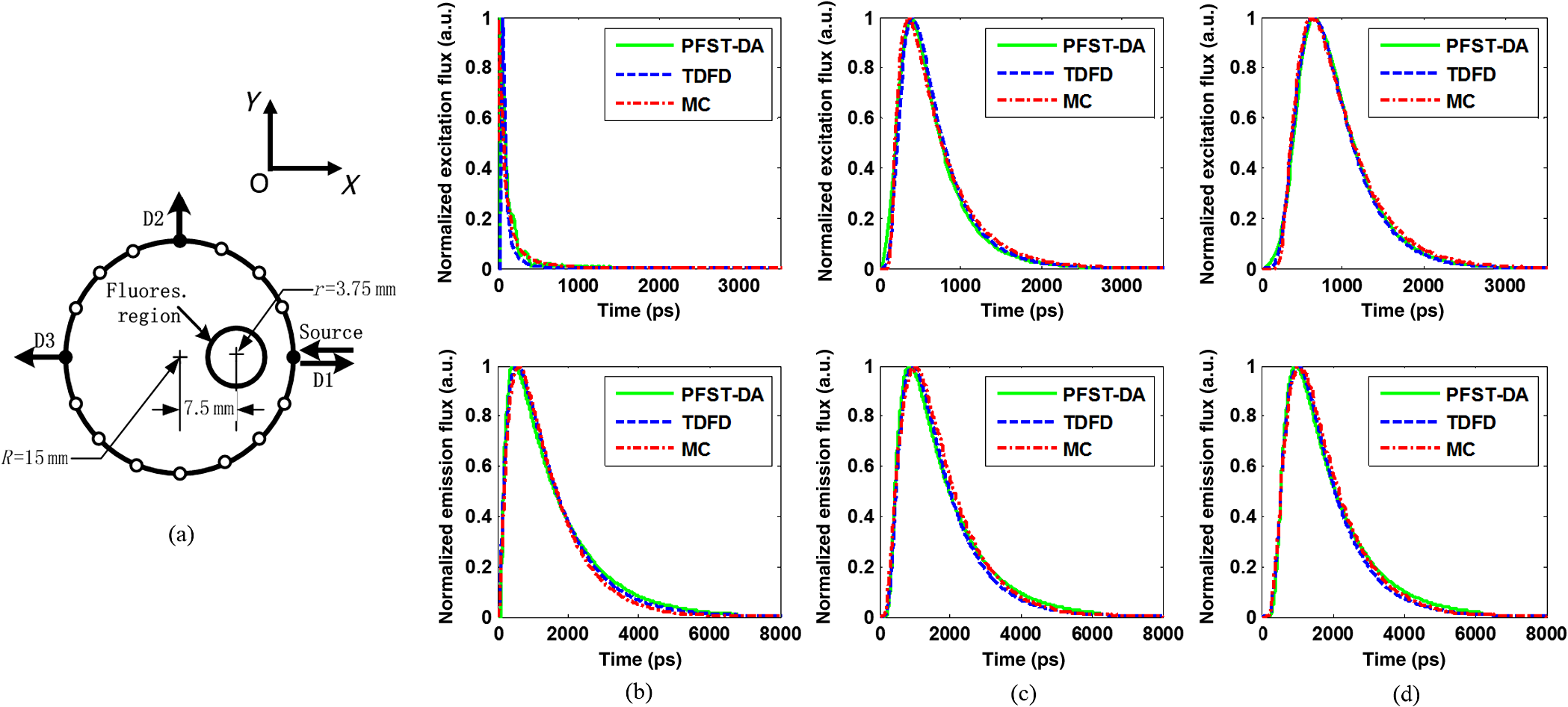

To investigate the accuracy of the parallelized Fourier-series truncated diffusion approximation (PFST–DA) in recovering the full TR data, we compare the normalized TPSF curves of the excitation and emission at the measuring sites, using the proposed PFST–DA, TDFD, and MC methods. According to the prior knowledge of the fluorescence MC simulation, the maximum flight times of the fluorescence signal at the farthest and nearest measuring positions are 8000 and 125 ps, respectively. Thus, the fundamental frequency is $π / 8000$ , and the total number of Fourier components is 64. To achieve an adequate accuracy of the forward calculation while avoiding an excess computational cost,¹¹ 400 temporal steps and $10^{10}$ photon packages are used for the TDFD solution and the GPU-accelerated fluorescence MC simulation, respectively. Figures 3(b)–3(d) are the normalized TPSF curves of the excitation and emission light at the measuring sites using the three methods. From left to right are the light detected at D1, D2, and D3, respectively. For the excitation light, the max relative errors of the PFST–DA method to the TDFD method and MC simulation at the three detection sites are $< 0.24$ and 0.2%, respectively. Although the emission results of the PFST–DA are a little worse than the excitation ones, the values are still within 0.35%. As to the computation time, the one with the PFST–DA scheme is 205.46 s, much less than that of the TDFD scheme by 2655.17 s.

To verify the accuracy of the selection criterion for the sampling frequencies, we assess the influence of the number of sampling frequencies on the forward calculation. A series of $N_{ω} = 20$ , 40, 64, and 160 sampling frequencies are used for the PFST–DA method with the detection site D2 shown in Fig. 3(a). Compared normalized TPSF curves for the excitation and emission light are shown in Figs. 4(a) and 4(b), respectively. The maximum relative difference between that of $N_{ω} = 64$ and that of $N_{ω} = 160$ is only 0.08%, which is considerably accurate. It is worth noting that, for assuring an adequate accuracy of the forward calculation without any excess computational cost, the number of the sampling frequencies is enough to be decided according to the selection criterion in Sec. 2.3.

Fig. 4

The normalized TPSFs of the (a) excitation and (b) fluorescent emission light by different numbers of sampling frequencies.

3.2.

Reconstruction Results from Simulations

The performance of the proposed method is evaluated for a cylinder background with a radius of $R = 15 mm$ and a length of $L = 40 mm$ , embedded with one and two fluorescence targets, called samples 1 and 2. A total of 64 coaxially aligned source–detector optodes are hierarchically and equally distributed around the cylinder by four layers at the horizontal planes of $Z = 5$ , 15, 25, and 35 mm. To make the simulated data realistic, the measurements are generated by a GPU-accelerated MC simulation with $10^{10}$ photon packages for each source radiation. We compare four reconstruction methods under the ART technique: the CW method with ART, the TDFD method with time-block ART (tTDFD), the PFST–DA method with time-block ART (tPFST–DA), and the PFST–DA method with frequency-block ART (fPFST–DA).

First, sample 1 is employed to compare the reconstruction results in terms of the maximum and the full width at half maximum (FWHM), respectively. The fluorescence target in sample 1 locates at ( $ρ = 7.5 mm$ , $θ = 0 \deg$ , $Z = 22.5 mm$ ) with a radius of $r = 2.5 mm$ and a length of $l = 15 mm$ . The reconstructed yield images at the horizontal slice of $Z = 22 mm$ and a vertical slice of $Y = 0 mm$ using the four reconstruction strategies with a target yield of $η μ_{a f}^{(T)} = 0.001 {mm}^{- 1}$ are shown in Fig. 5; so are the corresponding $X$ -profiles and $Z$ -profiles. Similarly, Figs. 6(a) and 6(b) and Figs. 6(c) and 6(d) are the corresponding profiles for the target yield of $η μ_{a f}^{(T)} = 0.002$ and $0.003 {mm}^{- 1}$ , respectively. Further comparisons among the four reconstruction strategies with respect to the reconstructed peak value and FWHM are shown in Table 1. It can be observed that the locations and sizes recovered by the three full TR methods are more in agreement with the true locations. The peak values of the tPFST–DA method at the three realistic targets are 2.16, 2.05, and 2.02%, a little lower than that with the tTDFD method, whereas in the fPFST–DA method, the values are 3.33, 4.26, and 4.58%, respectively. As for the computational time, it takes $\sim 624.56 \min$ for the tTDFD method to reconstruct the yield images, which is $\sim 1.15$ and 9.83 times those with the tPFST–DA and the fPFST–DA methods, respectively, at an approximate number of projection. The results reveal that, compared to the tTDFD method, the two PFST–DA methods can obtain the approximately accurate reconstructed images with much shorter computation time, especially with the fPFST–DA method.

Fig. 5

Reconstructed yield images and corresponding profiles of sample 1 at (a) $Z = 22 mm$ and (b) $Y = 0 mm$ by continuous wave (CW), time-domain finite-difference method with time-block algebraic reconstruction technique (tTDFD), parallelized Fourier-series truncated diffusion approximation method with time-block algebraic reconstruction technique (tPFST–DA), and PFST–DA method with frequency-block algebraic reconstruction technique (fPFST–DA) methods, with target yield of $0.001 {mm}^{- 1}$ .

Fig. 6

$X$ - and $Z$ -profiles of sample 1 at [(a) and (c)] $Z = 22 mm$ and [(b) and (d)] $Y = 0 mm$ by CW, tTDFD, tPFST–DA, and fPFST–DA methods, with target yield of [(a) and (b)] $0.002 {mm}^{- 1}$ and [(c) and (d)] $0.003 {mm}^{- 1}$ .

Table 1

Comparison among the four reconstruction methods for simulation scenarios of sample 1.

Method	Yield
	0.001 (mm−1)			0.002 (mm−1)		0.003 (mm−1)
	Peak value (mm−1)	FWHM- X/Z (mm)	Computation time (s)	Peak value (mm−1)	FWHM- X/Z (mm)	Peak value (mm−1)	FWHM- X/Z (mm)
CW	$8.0818 \times 10^{- 4}$	8.5/15.0	389.57	$1.6047 \times 10^{- 3}$	8.5/15.0	$2.4012 \times 10^{- 3}$	8.5/15.0
tTDFD	$9.8269 \times 10^{- 4}$	7.0/14.5	40,218.01	$1.9522 \times 10^{- 3}$	7.0/14.5	$2.9217 \times 10^{- 3}$	7.0/14.5
tPFST–DA	$9.6144 \times 10^{- 4}$	7.5/14.5	32,971.28	$1.9124 \times 10^{- 3}$	8.0/14.5	$2.8628 \times 10^{- 3}$	7.5/14.5
fPFST–DA	$9.5001 \times 10^{- 4}$	8.0/15.5	4071.36	$1.8690 \times 10^{- 3}$	8.0/15.0	$2.7878 \times 10^{- 3}$	7.5/14.5

Note: CW, continuous wave; tTDFD, time-domain finite-difference method with time-block algebraic reconstruction technique; tPFST-DA, parallelized Fourier-series truncated diffusion approximation method with time-block algebraic reconstruction technique; fPFST–DA, PFST–DA method with frequency-block algebraic reconstruction technique.

For sample 2, the two fluorescence targets are with the same radius and length as that in sample 1 at the locations of ( $θ = 0 \deg$ , $Z = 22.5 mm$ ) and ( $θ = 180 \deg$ , $Z = 12.5 mm$ ), under a fixed target fluorescent properties of $η μ_{a f}^{(T)} = 0.001 {mm}^{- 1}$ . To compare the four reconstruction methods by the spatial resolution, the center-to-center separations (CCS) of the two targets are set as 8, 11, and 14 mm, respectively, with a measure defined as $R = [{(η μ_{a f})}_{\max} - {(η μ_{a f})}_{(x = 0 mm)}] / [{(η μ_{a f})}_{\max} - {(η μ_{a f})}_{\min}]$ in the $X$ -profile of the reconstructed yield image. Figures 7 Fig. 8–9 illustrate the reconstructed yield images at the horizontal slice of $Z = 18 mm$ and a vertical slice of $Y = 0 mm$ , with the corresponding profiles along the $X$ axis and $Z$ axis. Further comparison among the four reconstruction strategies is shown in Table 2. The images in Figs. 7 and 8 reveal that the tTDFD method can best separate the two targets, similar to the tPFST–DA and the fPFST–DA methods, and much better than the CW method. This is because the tTDFD method carries the richest and truest information about the targets. As of Fig. 9 where $CCS = 14 mm$ , the spatial resolution by the fPFST–DA method is the highest, where the spatial resolutions of the two PFST–DA methods are even 0.64 and 3.53% better than that of the tTDFD method, respectively, which may be explained as the reconstruction quality of ART algorithm is related to an optimal iteration number and relaxing factor. In this situation, the parameters are more fit for the fPFST–DA method.

Fig. 7

Reconstructed yield images and corresponding profiles of sample 2 at (a) $Z = 18 mm$ and (b) $Y = 0 mm$ by CW, tTDFD, tPFST–DA, and fPFST–DA methods, with center-to-center separation $(CCS) = 14 mm$ .

Fig. 8

Reconstructed yield images and corresponding profiles of sample 2 at (a) $Z = 18 mm$ and (b) $Y = 0 mm$ by CW, tTDFD, tPFST–DA, and fPFST–DA methods, with 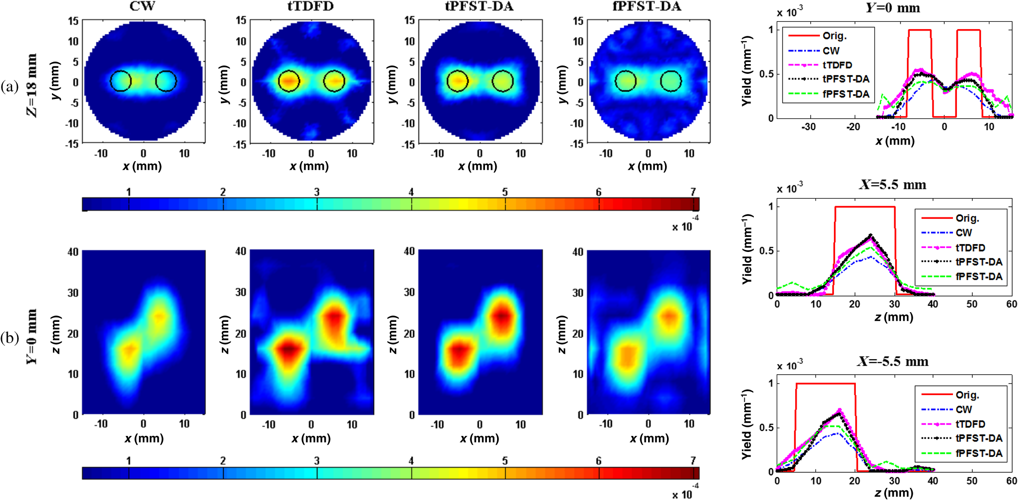$CCS = 11 mm$ .

Fig. 9

Reconstructed yield images and corresponding profiles of sample 2 at (a) $Z = 18 mm$ and (b) $Y = 0 mm$ by CW, tTDFD, tPFST–DA, and fPFST–DA methods, with 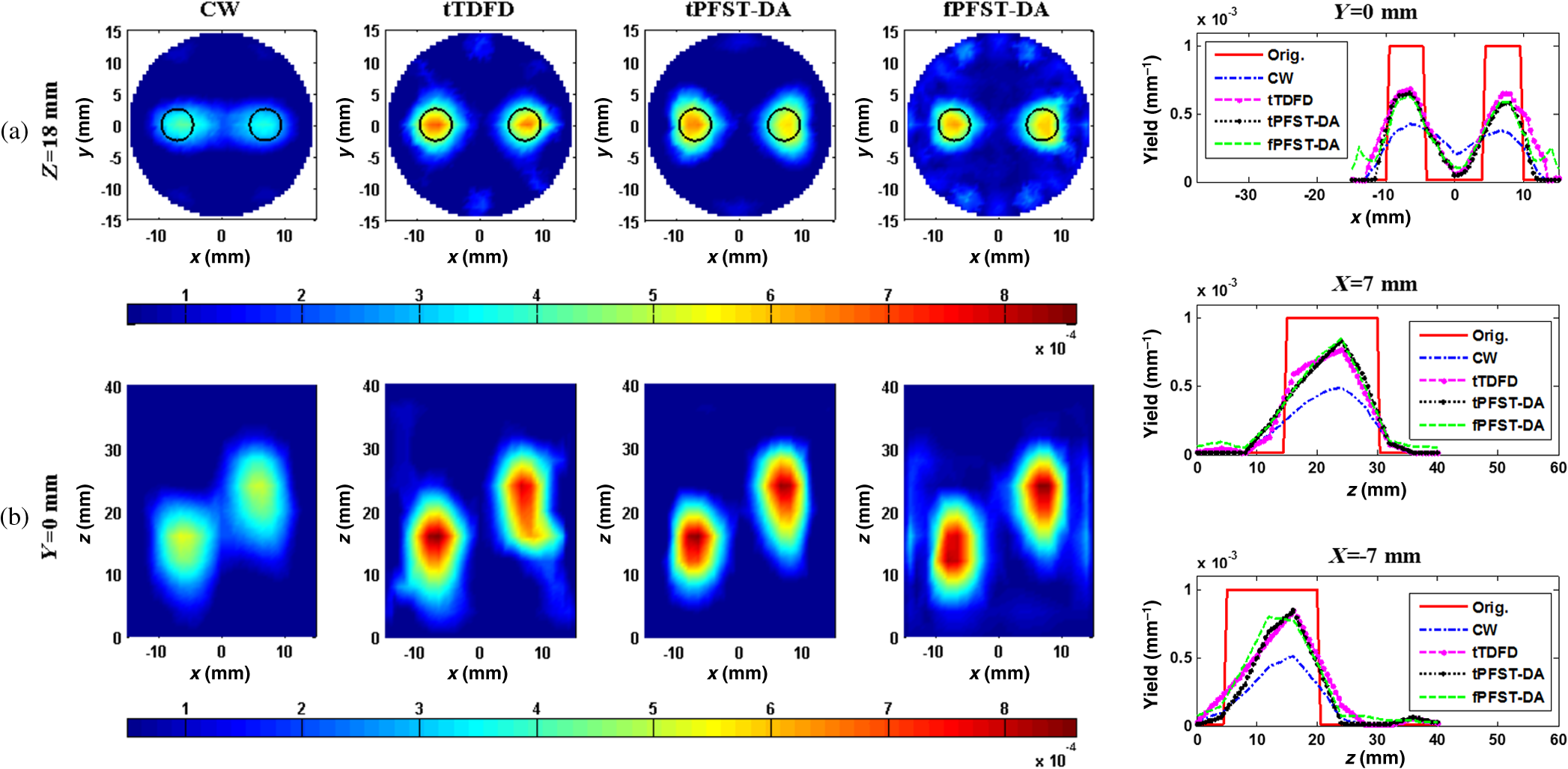$CCS = 8 mm$ .

Table 2

Comparison among the four reconstruction methods for simulation scenarios of sample 2.

Method	CCS
	14 (mm)		11 (mm)		8 (mm)
	Peak value left/right (mm−1)	R	Peak value left/right (mm−1)	R	Peak value left/right (mm−1)	R
CW	$5.3406 \times 10^{- 4} / 5.1345 \times 10^{- 4}$	0.5205	$4.8363 \times 10^{- 4} / 4.7913 \times 10^{- 4}$	0.2053	$4.9975 \times 10^{- 4} / 4.9100 \times 10^{- 4}$	0.1073
tTDFD	$8.6000 \times 10^{- 4} / 7.8663 \times 10^{- 4}$	0.9294	$7.0558 \times 10^{- 4} / 6.4973 \times 10^{- 4}$	0.4760	$7.4114 \times 10^{- 4} / 6.4996 \times 10^{- 4}$	0.2131
tPFST–DA	$8.5501 \times 10^{- 4} / 8.3843 \times 10^{- 4}$	0.9358	$6.6754 \times 10^{- 4} / 6.8690 \times 10^{- 4}$	0.4516	$7.0443 \times 10^{- 4} / 7.0179 \times 10^{- 4}$	0.1961
fPFST–DA	$8.1069 \times 10^{- 4} / 8.5000 \times 10^{- 4}$	0.9647	$5.6056 \times 10^{- 4} / 5.7478 \times 10^{- 4}$	0.4377	$5.6939 \times 10^{- 4} / 5.8947 \times 10^{- 4}$	0.1993

Note: CCS, center-to-center separation.

3.3.

Reconstruction Results from Experiments

To validate the proposed method, a time-correlated single photon counting (TCSPC) system is employed to perform a series of TD phantom experiments. As shown in Fig. 10, the light source in the setup is a picosecond-pulsed laser system that employs a programmable controller (PDL828, PicoQuant, Germany) to drive 780 nm [the peak excitation wavelength of indocyanine green (ICG)] fiber-coupled 70 ps pulsed laser diode heads (LDH-P-P-780, PicoQuant, Germany). The output beam is distributed to $16 62.5 μ m$ source fibers by a $1 \times 16$ fiber switch for the tissue scanning. The emergent photons are collected by $500 μ m$ detection fibers placed at 16 sites equally spaced around the phantom boundary on the imaging plane, in which only measurements from the 11 detectors opposite to each of the 16 sources are employed for the image reconstruction. Then the collected photons are delivered to a photomultiplier tube (PMT) photon-counting header (PMC-100, Becker&Hickl, Germany) and temporally resolved by a TCSPC module (SPC-134, Becker&Hickl, Germany). In front of the PMT detector mounts a six-hole filter wheel (FW103B, Thorlabs) that houses four neutral density filters with the optical densities of 1 to 4, respectively, and a bandpass filter (ICG-A Emitter, Semrock). To facilitate the deployment of the fibers and the modeling of the light propagation, the output ends of 16 source fibers and input ends are paired into 16 coaxial optodes.

Fig. 10

(a) Schematic diagram and (b) photo of the used time-correlated single photon counting system.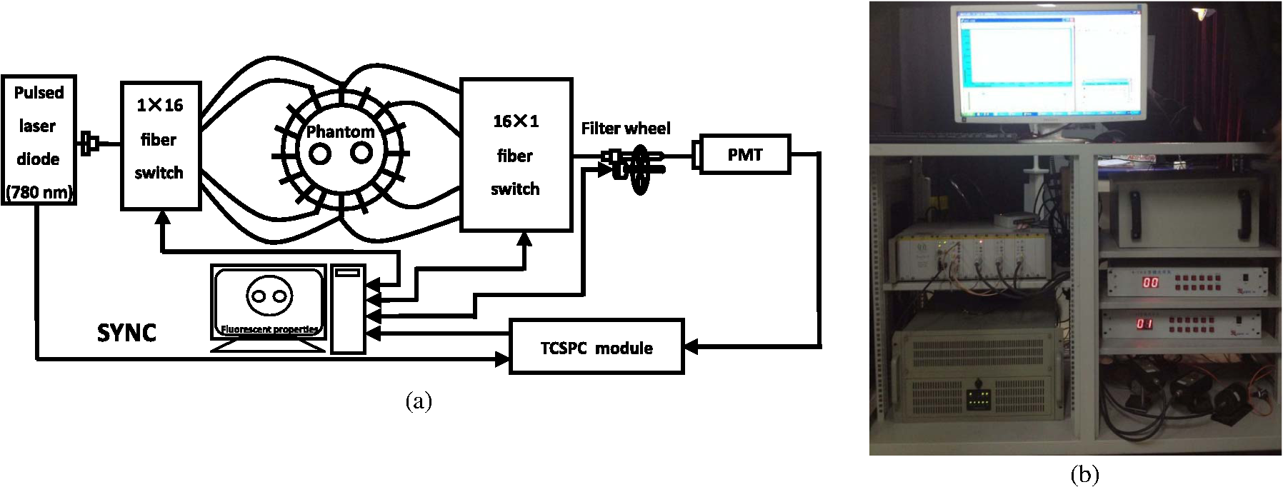

For the TCSPC setup, the output of a time-to-amplitude converter is sampled into 4096 time bins with a width of $Δ T_{b} = 17.114 ps$ . The acquisition periods of the excitation and emission signals are adjusted to satisfy a suitable signal-to-noise ratio (SNR) respectively, within the scope of the effective counting rate.¹⁶ To prevent the overflow of the Born-normalized TR data and also assure an adequately high SNR, time ranges of the excitation and emission TPSFs where the sample intensities are $> 20 %$ of their respective maximum are decided, and their intersection is chosen for the reconstructions. For the full use of the TR information, the gate interval in the overlap time-gating method is set to the time-bin width of the measured TPSF, while the gating width is set to 100 gate intervals.

To simulate the fluorescent targets embedded in the tissue, a 5-mm-diameter cylindrical hole is drilled into a 30-mm-diameter cylindrical phantom made from polyformaldehyde and filled with a mixture of 1% Intralipid solution and ICG concentration of $\sim 100 nM$ , leading to a fluorescent yield of $η μ_{a f} = 0.001 {mm}^{- 1}$ . The absorption and the reduced scattering coefficients of the targets are assumed to be equal at both the excitation and emission wavelengths, and determined to be the same as the background ones with $μ_{a x} = μ_{a m} = 0.0038 {mm}^{- 1}$ and $μ_{s x} = μ_{s m} = 0.978 {mm}^{- 1}$ , respectively, by the TR spectroscopy technique,¹⁹ while the initial background fluorescent yield is empirically set to $η μ_{a f} = 1 \times 10^{- 5} {mm}^{- 1}$ , and the lifetime is kept as a constant of $τ = 560 ps$ for both the background and targets. Similar to the simulative investigations, 400 temporal steps and 64 sampling frequencies are used for the TDFD solution and the PFST–DA methods, respectively.

Figure 11 shows the reconstructed yield images at the horizontal slice of $Z = 30 mm$ and the corresponding $X$ -profiles using the CW, tTDFD, tPFST–DA, and fPFST–DA reconstruction strategies. It is obvious that the locations and quantitative nature of the two targets are more in good agreement with the true targets for the three TD schemes than those with the CW scheme. Further quantitative details about the reconstructed peak value of the two targets and the spatial resolution are shown in Table 3. Compared to the tTDFD method, the maximum relative difference of the peak value by the two PFST–DA methods is $\sim 5.86 %$ . As to the spatial resolution, the relative errors are 3.29 and 4.96% for the tPFST–DA and the fPFST–DA methods, respectively. The computation time of the PFST–DA method in the forward calculation is 54.48 s, $< 10 %$ that of the tTDFD method with 587.32 s. Although the reconstruction time of the tPFST–DA method is similar to that of the TDFD time of 147.98 min, that of the fPFST–DA method is only 15.31 min, $\sim 10.35 %$ that of the latter. All the observations confirm to those in the simulative investigations.

Fig. 11

Reconstructed (a) 2-D yield images and (b) corresponding profiles by CW, tTDFD, tPFST–DA, and fPFST–DA methods.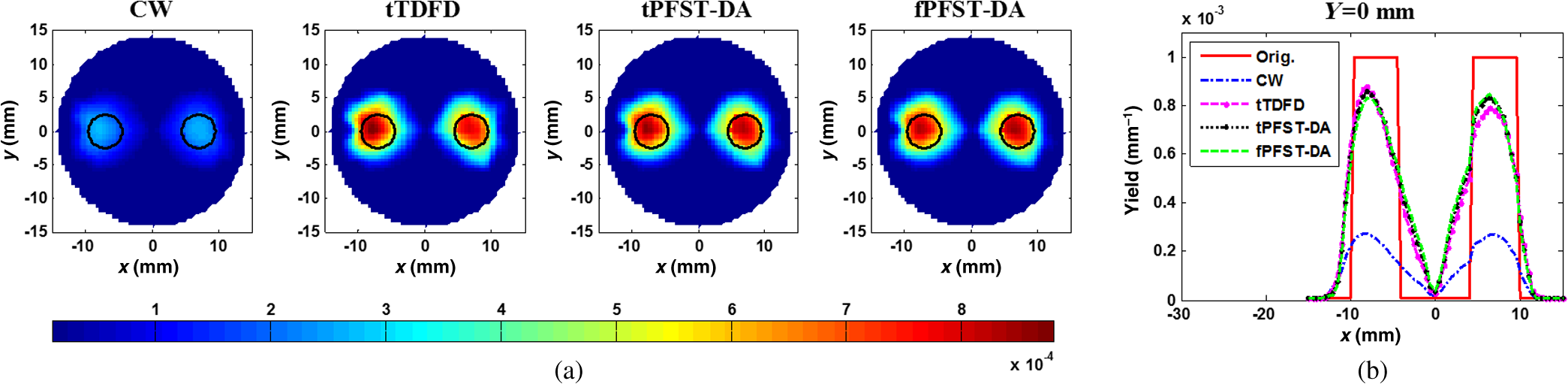

Table 3

Comparison among the four reconstruction methods for experimental scenarios.

Method		CW	tTDFD	tPFST–DA	fPFST–DA
Peak value ( ${mm}^{- 1}$ )	Left	$1.7028 \times 10^{- 4}$	$5.1047 \times 10^{- 4}$	$5.2001 \times 10^{- 4}$	$5.1870 \times 10^{- 4}$
Peak value ( ${mm}^{- 1}$ )	Right	$1.9036 \times 10^{- 4}$	$5.5383 \times 10^{- 4}$	$5.7754 \times 10^{- 4}$	$5.8350 \times 10^{- 4}$
Spatial resolution $R$		0.2587	0.8575	0.8293	0.8150
Computation time (s)		132.19	9479.11	8948.23	990.37

4. Discussion and Conclusions

We propose in this paper a parallelized Fourier-series truncated DA for the full TR–DFT image reconstruction. In this computationally efficient scheme, the time-dependent photon density is expanded to a Fourier series and the TD–DE is calculated by solving the independent FD–DEs at multiple sampling frequencies, with the support of a combined multicore CPU-based coarse-grain and multithread GPU-based fine-grain parallelization strategy. Based on this forward model, both the TD and FD inversion procedures are developed under the framework of block ART, referred to as the tPFST–DA and fPFST–DA methods, respectively.

The forward resulting TPSF curves are tested by comparison with those from the TDFD solution and the TD MC simulation. The reconstructions are validated for their quantitativeness and spatial resolution by both simulations and phantom experiments. Results show that the proposed method can generate reconstructions comparable to the explicit TD scheme, with significantly reduced computational time, especially by the fPFST–DA method.

According to the studies done in Ref. 19, the advantage of the truncated Fourier-series method mainly lies in the far fewer number of frequency components needed than the temporal steps in the tTDFD scheme. With the aforementioned accelerating strategy, the truncated Fourier-series scheme is more suitable to be applied to the full TR–DFT reconstruction of 3-D or larger-sized tissues that require more frequency components for an accurate approximation. However, in the experimental measurements, due to the large differentiation of the impulse response function curve of individual fiber switching channel and the fact of manual switching of fibers needed in the current setup, the workload to accurately obtain all the instrument response function curves was significantly increased. Considering the measuring time and system stability, the experimental validations were performed in a 2-D mode.

It should be pointed out that the calculations of stiffness and Jacobian matrices in the TDFD method are executed in the same fine-grain parallelization strategy as the PFST–DA method, while every time step is performed in a recursive way, leading to no coarse-grain parallelization mechanism. Moreover, although there is a potential of using the block iterative algorithms on a parallel architecture, such as a multicore CPU or multithread GPU, the block ART iteration needs $N_{ω}$ times storage space of that in a conventional ART algorithm, to move the Jacobian matrix into and execute the calculation in the GPU device memory, which makes it difficult to effectively execute in the device memory.

Acknowledgments

The authors acknowledge the funding support from the National Natural Science Foundation of China (81271618, 81371602, 61475115, 61475116, and 81401453), Tianjin Municipal Government of China (13JCZDJC28000, 14JCQNJC14400, and 15JCZDJC31800), the Research Fund for the Doctoral Program of Higher Education of China (20120032110056), and the 111 project (B07014).

References

1.

E. M. Sevick-Muraca, J. P. Houston and M. Gurfinkel, “Fluorescence-enhanced, near infrared diagnostic imaging with contrast agent,” Curr. Opin. Chem. Biol., 6 642 –650 (2002). http://dx.doi.org/10.1016/S1367-5931(02)00356-3 COCBF4 1367-5931 Google Scholar

2.

A. B. Milstein et al., “Fluorescence optical diffusion tomography,” Appl. Opt., 42 3081 –3094 (2003). http://dx.doi.org/10.1364/AO.42.003081 APOPAI 0003-6935 Google Scholar

3.

T. Dutduran et al., “Diffuse optics for tissue monitoring and tomography,” Rep. Prog. Phys., 73 076701 (2010). http://dx.doi.org/10.1088/0034-4885/73/7/076701 RPPHAG 0034-4885 Google Scholar

4.

A. Gibson and H. Dehghani, “Diffuse optical imaging,” Phil. Trans. R. Soc. A, 367 3055 –3072 (2009). http://dx.doi.org/10.1098/rsta.2009.0080 PTRMAD 1364-503X Google Scholar

5.

F. Leblond et al., “Pre-clinical whole-body fluorescence imaging: review of instruments, method and applications,” J. Photochem. Photobiol. B: Biol., 98 77 –94 (2010). http://dx.doi.org/10.1016/j.jphotobiol.2009.11.007 JPPBEG 1011-1344 Google Scholar

6.

C. Darne, Y.-J. Lu and E. M. Sevick-Muraca, “Small animal fluorescence and bioluminescence tomography: a review of approaches, algorithms and technology update,” Phys. Med. Biol., 59 R1 –R64 (2014). http://dx.doi.org/10.1088/0031-9155/59/1/R1 PHMBA7 0031-9155 Google Scholar

7.

A. T. N. Kumar et al., “Comparison of frequency-domain and time-domain ﬂuorescence lifetime tomography,” Opt. Lett., 33 470 –472 (2008). http://dx.doi.org/10.1364/OL.33.000470 OPLEDP 0146-9592 Google Scholar

8.

V. Venugopa et al., “Full-field time-resolved fluorescence tomography of small animals,” Opt. Lett., 35 3189 –3191 (2010). http://dx.doi.org/10.1364/OL.35.003189 OPLEDP 0146-9592 Google Scholar

9.

A. T. N. Kumar et al., “Time-resolved fluorescence tomography of turbid media based on lifetime contrast,” Opt. Express, 14 12255 –12270 (2006). http://dx.doi.org/10.1364/OE.14.012255 OPEXFF 1094-4087 Google Scholar

10.

S. R. Arridge et al., “A finite element approach for modeling photon transport in tissue,” Med. Phys., 20 299 –309 (1993). http://dx.doi.org/10.1118/1.597069 MPHYA6 0094-2405 Google Scholar

11.

F. Gao et al., “A self-normalized, full time-resolved method for fluorescence diffuse optical tomography,” Opt. Express, 16 13104 –13121 (2008). http://dx.doi.org/10.1364/OE.16.013104 OPEXFF 1094-4087 Google Scholar

12.

Q. Zhu et al., “A three-dimensional finite element model and image reconstruction algorithm for time-domain fluorescence imaging in highly scattering media,” Phys. Med. Biol., 56 7419 –7434 (2011). http://dx.doi.org/10.1088/0031-9155/56/23/006 PHMBA7 0031-9155 Google Scholar

13.

F. Leblond et al., “Toward whole-body optical imaging of rats using single-photon counting fluorescence tomography,” Opt. Lett., 36 3723 –3725 (2011). http://dx.doi.org/10.1364/OL.36.003723 OPLEDP 0146-9592 Google Scholar

14.

V. Venugopal and X. Intes, “Adaptive wide-field optical tomography,” J. Biomed. Opt., 18 036006 (2013). http://dx.doi.org/10.1117/1.JBO.18.3.036006 JBOPFO 1083-3668 Google Scholar

15.

A. Corlu et al., “Three-dimensional in vivo fluorescence diffuse optical tomography of breast cancer in humans,” Opt. Express, 15 6696 –6716 (2007). http://dx.doi.org/10.1364/OE.15.006696 OPEXFF 1094-4087 Google Scholar

16.

W. Zhang et al., “Combined time-domain hemoglobin and fluorescence diffuse optical tomography for breast tumor diagnosis: a methodological study,” Biomed. Opt. Express., 4 331 –348 (2013). http://dx.doi.org/10.1364/BOE.4.000331 BOEICL 2156-7085 Google Scholar

17.

R. W. Holt et al., “Multiple-gate time domain diffuse fluorescence tomography allows more sparse tissue sampling without compromising image quality,” Opt. Lett., 37 2559 –2561 (2012). http://dx.doi.org/10.1364/OL.37.002559 OPLEDP 0146-9592 Google Scholar

18.

S. Lam, F. Lesage and X. Intes, “Time-domain fluorescent diffuse optical tomography: analytical expressions,” Opt. Express, 13 2263 –2275 (2005). http://dx.doi.org/10.1364/OPEX.13.002263 OPEXFF 1094-4087 Google Scholar

19.

F. Gao et al., “A linear, featured-data scheme for image reconstruction in time-domain fluorescence molecular tomography,” Opt. Express, 14 7109 –7124 (2006). http://dx.doi.org/10.1364/OE.14.007109 OPEXFF 1094-4087 Google Scholar

20.

M. Schweiger and S. R. Arridge, “Application of temporal filters to time resolved data in optical tomography,” Phys. Med. Biol., 44 1699 –1717 (1999). http://dx.doi.org/10.1088/0031-9155/44/7/310 PHMBA7 0031-9155 Google Scholar

21.

J. Li et al., “Overlap time-gating approach for improving time-domain diffuse fluorescence tomography based on the IRF-calibrated Born normalization,” Opt. Lett., 38 1841 –1843 (2013). http://dx.doi.org/10.1364/OL.38.001841 OPLEDP 0146-9592 Google Scholar

22.

A. Pulkkinen and T. Tarvainen, “Truncated Fourier-series approximation of the time-domain radiative transfer equation using finite elements,” J. Opt. Soc. Am. A, 30 470 –478 (2013). http://dx.doi.org/10.1364/JOSAA.30.000470 JOAOD6 0740-3232 Google Scholar

23.

R. Ziegler et al., “Nonlinear reconstruction of absorption and fluorescence contrast from measured diffuse transmittance and reflectance of a compressed-breast-simulating phantom,” Appl. Opt., 48 4651 –4662 (2009). http://dx.doi.org/10.1364/AO.48.004651 APOPAI 0003-6935 Google Scholar

24.

F. Gao, H. Zhao and Y. Yamada, “Improvement of image quality in diffuse optical tomography by use of full time-resolved data,” Appl. Opt., 41 778 –791 (2002). http://dx.doi.org/10.1364/AO.41.000778 APOPAI 0003-6935 Google Scholar

25.

O. C. Zienkiewicz and R. L. Taylor, The Finite Element Methods Volume, 15th ed.Elsevier Pte Ltd., Singapore (2004). Google Scholar

26.

P. P. B. Eggermont, G. T. Herman and A. Lent, “Iterative algorithms for large partitioned linear systems, with applications to image reconstruction,” Linear Algebra Appl., 40 37 –67 (1981). http://dx.doi.org/10.1016/0024-3795(81)90139-7 LAAPAW 0024-3795 Google Scholar

27.

X. Yi et al., “GPU-accelerated Monte-Carlo modeling for fluorescence propagation in turbid medium,” Proc. SPIE, 8216 82160U (2012). http://dx.doi.org/10.1117/12.902988 PSISDG 0277-786X Google Scholar

28.

X. Yi et al., “Full domain-decomposition scheme for diffuse optical tomography of large-sized tissues with a combined CPU and GPU parallelization,” Appl. Opt., 53 2754 –2765 (2014). http://dx.doi.org/10.1364/AO.53.002754 APOPAI 0003-6935 Google Scholar

Biography

Xi Yi is a PhD of biomedical engineering at the Biomedical Photonic Imaging Laboratory of Tianjin University. Her research is focused on diffuse optical tomography and diffuse fluorescence tomography. She is focused on developing advanced optical imaging methods to improve the quality of large-sized or three-dimensional image reconstructions on the base of certain acceleration method.

Biographies for the other authors are not available.

Citation Download Citation

Xi Yi, Bingyuan Wang, Wenbo Wan, Yihan Wang, Yanqi Zhang, Huijuan Zhao, and Feng Gao "Full time-resolved diffuse fluorescence tomography accelerated with parallelized Fourier-series truncated diffusion approximation," Journal of Biomedical Optics 20(5), 056003 (12 May 2015). https://doi.org/10.1117/1.JBO.20.5.056003

Published: 12 May 2015

Access the abstract

JOURNAL ARTICLE
11 PAGES

DOWNLOAD PAPER SAVE TO MY LIBRARY

GET CITATION

CITATIONS

Cited by 3 scholarly publications.

Explore citations on Lens.org

RIGHTS & PERMISSIONS

Get copyright permission Get copyright permission on Copyright Marketplace

KEYWORDS

Diffusion

Fluorescence tomography

Continuous wave operation

Reconstruction algorithms

Atrial fibrillation

Spatial resolution

Tissues

1.

Introduction

2.

Methods

2.1.

Fourier-Series Truncated DE for Full TR Data

Eq. (1)

Eq. (2)

Eq. (3)

2.2.

Full TR–DFT Method with Fourier-Series Truncated DE

Eq. (4)

Fig. 1

2.3.

Selection for the Sampling Frequency

2.4.

Parallelization Strategy

Eq. (5)

Fig. 2

3.

Results

3.1.

Forward Results from Simulations

Fig. 3

Fig. 4

3.2.

Reconstruction Results from Simulations

Fig. 5

Fig. 6

Table 1

Fig. 7

Fig. 8

Fig. 9

Table 2

3.3.

Reconstruction Results from Experiments

Fig. 10

Fig. 11

Table 3

4.

Discussion and Conclusions

Acknowledgments

References

Biography

Show All Keywords

Keywords/Phrases

Search In:

Publication Years