1.

Introduction

Functional near-infrared spectroscopy (fNIRS) is a noninvasive optical imaging technique which measures the absorption of near-infrared light between 650 and 950 nm through the intact skull. Since the absorption spectra of oxygenated hemoglobin (HbO) and deoxygenated hemoglobin (Hb) are different, the concentration change of hemoglobin in vivo can be estimated from spectral recordings.^1,2 fNIRS technology has been developing rapidly and gaining popularity as a tool for functional neuroimaging due to its ability to measure cerebral hemodynamic changes associated with functional brain activity.^3,4

Compared with functional magnetic resonance imaging (fMRI), fNIRS has several advantages including relatively low cost, portability, higher temporal resolution, and continuous measurement over longer time periods. In addition, fNIRS does not require participants to lie in a confined space with their heads fixed. These advantages allow fNIRS to be widely applied in different populations and experimental or clinical conditions such as in the study of infants and children,^5,6 cognition,⁷ motor tasks,⁸ brain stimulation,^9,10 and brain disorder patients.^11,12 As we know, the signals recorded from participants mentioned above, especially children and patients, usually contain many motion artifacts. If these motion artifacts are not removed or inhibited, analysis results are not convincing. Therefore, how to avoid motion artifacts is a very important issue.

With the improvement in fNIRS technology, although fNIRS is more tolerant of head motion and robust to motion artifacts than fMRI,^4,13 it is still difficult to completely avoid motion artifacts. When participants move their heads, motion artifacts still often influence the fNIRS signal.^14,15 Thus, motion correction is a key step before further analysis of fNIRS recordings.

To address this important issue, a number of methods have been proposed. Motion correction methods can generally be divided into two categories: (a) those that require external signals; and (b) those that do not.

For the first category, the external signals should be highly sensitive to motion artifacts but not to brain activity such as those recorded from an fNIRS channel with a very short emitter–receiver distance^16,17 or an accelerometer.¹⁸ In this case, adaptive filtering is used for motion correction. The drawback of this approach is that the adaptive filter cannot completely remove motion artifacts if the information about motion contained in the external signals is not exact.

In the second category, spline interpolation (SI),¹⁹ wavelet filtering (WF),²⁰ and kurtosis-based wavelet filtering (kbWF)¹⁴ are commonly used as motion correction methods. In previous studies, these methods performed well.^14,15,21 However, there are also some limits in their practical application. For example, SI needs the setting of many parameters; WF and kbWF are poor for the correction of baseline shifts.¹⁴ In this study, we propose a motion correction method that can be applied to standard datasets without any external signal.

It is well known that the brain is a complex, dynamic system. fNIRS signals exhibit strong nonstationarity.¹⁹ Thus, we propose a motion correction method based on empirical mode decomposition (EMD), which was first proposed by Huang et al.²² The EMD can be used to break down signals into various components, called as intrinsic mode functions (IFMs), and these components form a complete and nearly orthogonal basis for the original signal. Since the EMD is based on the local characteristic time scale of the data, it can be applied to nonlinear and nonstationary processes. Currently, the EMD has been widely used for analyzing physiological signals such as electroencephalogram, magnetoencephalogram, and blood–oxygen-level-dependent signal,^23–27 including the noise reduction in these signals.²⁸ In this study, we propose to reduce the motion artifacts in the fNIRS recordings using the EMD.

To estimate the performance of the proposed EMD-based method and to compare it with other methods (SI, WF, and kbWF), we used simulated data in a procedure based on previous work.^14,15,21,29 Real motion artifacts are complex and variable, and difficult to simulate,²¹ so real resting-state fNIRS data contaminated by motion artifacts were used as the noise. A synthesized hemodynamic response function (HRF) was used as the true hemodynamic response (true signal). Knowing the true hemodynamic response, we can calculate metrics which quantitatively compare the performance of different motion correction methods.

2.

Materials and Methods

2.1.

Resting-State Functional Near-Infrared Spectroscopy Data

Thirteen children (6 females and 7 males, aged 6 to 9 years, $\text{mean}\pm \text{standard deviation}$ $7.3\pm 1.1$) took part in this study after their parents provided informed consent. This study was approved by the ethics committee of the State Key Laboratory of Cognitive Neuroscience and Learning at the Beijing Normal University. Information of all participants is summarized in Table 1. The data were collected using a resting-state paradigm, in which the participants were instructed to relax in a seated position in front of a 19-in. monitor and to try not to think of anything. Five minutes of resting-state fNIRS data were collected from each participant.

Table 1

Information of the subjects.

Subject no.	Sex	Age
1	Male	6
2	Female	9
3	Male	8
4	Male	6
5	Male	6
6	Female	7
7	Male	8
8	Female	7
9	Male	7
10	Female	6
11	Male	8
12	Female	9
13	Female	8

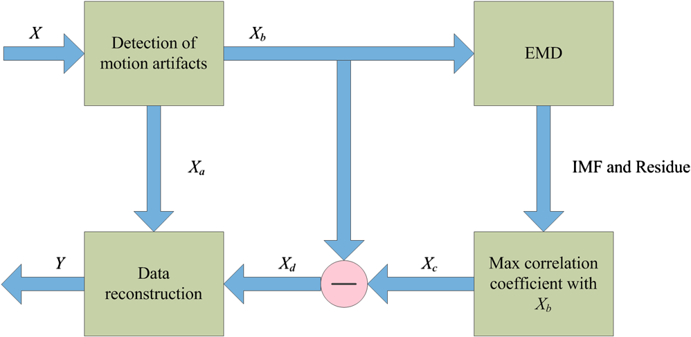
In this study, we used an ETG-4000 (Hitachi Medical Company, Japan) NIRS system to measure the relative concentration changes in HbO and Hb. We used a single $3\times 11$ measurement patch, which was placed symmetrically over each participant’s frontal cortex, wrapping around and covering the temporal cortex (Fig. 1). In this patch, 17 emitters and 16 detectors were positioned in an alternating fashion, forming 52 measurement channels. The absorption of near-infrared light at wavelengths 695 and 830 nm was measured at a sampling rate of 10 Hz.

Fig. 1

(a) A photo of the experimental setup; and (b) fNIRS probe locations mapped to a brain model.

Since the participants were children, motion artifacts were common, despite them being instructed not to move their heads during recording. We obtained 676 channels of data ($13\text{subjects}\times 52\text{channels}$) in total. Following warnings from the built-in diagnostics of the ETG-4000 system and by visual inspection, the data from 164 channels were thrown out, and the remaining 512 channels were used for further analysis. In this study, we only used the HbO data.

2.3.

Motion Correction Methods

2.3.1.

Empirical mode decomposition-based motion correction method

EMD is a method that breaks down signals into a collection of intrinsic mode functions (IMFs). An IMF is a function that satisfies two conditions: (a) in the whole dataset, the number of extrema and the number of zero crossings must be the same or differ at most by one; and (b) at any point in the dataset, the mean value of the envelope defined by the maxima and the envelope defined by the minima must be zero.²²

EMD is implemented using a sifting process that uses only local extrema. There are some steps taken to calculate the IMF of a given data. The first step is to find all the local maxima and minima over the whole data. Next, all the local maxima are connected by a cubic spline as the upper envelope. The same process is repeated for the local minima to produce the lower envelope. The second step is to calculate the average of the two envelopes $m$ and to subtract $m$ from the original data, resulting in new data $h=r_0-m$, where $r_0$ is equal to $x$ which is the original data. This data $h$ repeat above steps until $h$ satisfies the conditions of an IMF. The current data $h$ becomes the first IMF designated as $c_1$. Then the above steps are repeated on the residual $r_1=r_0-c_1$. The sifting process stops until no more IMF can be extracted from the residual $r_n$. The original data $x$ can be reconstructed as

Eq. (1)

$$x=\sum _{j=1}^n{c}_j+r_n,$$

where $r_n$ is the residual after $n$ IMFs are extracted.

We propose a motion correction method based on EMD. Our procedure is similar to the spline interpolation method.¹⁹ The main idea is that the IFM from the EMD that is most similar to the motion artifact contaminated signal approximates the motion artifact. Thus, we subtract the most similar IMF from the signal to remove the motion artifact. The five data processing steps of our method are as follows. (a) Apply a motion artifact detection method to segment the data into time periods which have motion artifact and which do not. The method provides reliable detection of motion artifacts based on changes in signal amplitude or standard deviation. If the standard deviation or the peak-to-peak amplitude exceeds the preset thresholds (SDThresh and AMPThresh) within a time window of length $t$, the data from the beginning of that window to $T$ seconds later are defined as motion artifact.³ (b) Perform an EMD on the time periods detected as having motion artifact, each segment separately. (c) Calculate the correlation coefficients between each IMF (including residue here) and the original data. (d) Subtract the IMF (or residue) with the largest correlation coefficient from the original data. (e) Reassemble the whole time series by concatenating the segments. To ensure continuity of the HbO signal across segment boundaries, we use the method proposed in Ref. 19: shift the HbO values in each segment by a constant HbO value that is determined by the mean of the segment and the mean of the previous segment. The detailed description of this step can be found in Ref. 19.

The flowchart of this procedure is shown in Fig. 2. In order to detect the motion artifact periods, we set the parameters following previous work:^14,15,29 $\mathrm{SDThresh}=20$, $\mathrm{AMPThresh}=0.5$, $t=0.5$, and $T=2$.

Fig. 2

Flowchart of the EMD motion correction method. $X$: original data, $X_a$: segments of $X$ without motion artifacts, $X_b$: segments of $X$ with motion artifacts, $X_c$: IMF or residue with largest correlation to $X_b$, $X_d=X_b-X_c$, and $Y$: corrected data.

2.3.2.

Spline interpolation

The SI method compared here was proposed by Scholkmann et al.¹⁹ The main idea is that the spline fit to the raw signal during time periods when artifact is detected approximates the motion artifact, since artifacts are large compared with the physiological signals. Thus, subtracting the spline from the raw signal removes the artifact. The time periods with motion artifact are automatically detected using the same method described in EMD step (a). Then each of the periods is modeled separately by a cubic spline. Next, the spline is subtracted from the original data. The time series is then reconstructed by reassembling the artifact time periods, together with the time periods without artifact. To ensure continuity of signal, the procedure detailed in Ref. 19 [the same as EMD step (e)] is used.

The parameters of the motion artifact detection method were set to the same values as those in the EMD method. In addition, a parameter $p$ that determines the degree of the SI needs to be set. When $p=0$, the smoothing spline is the least-squares straight line fit to the data, while when $p=1$, it is the natural cubic SI. In this study, we set $p=0.9$ to 0.99 and chose the best results for comparison with the other methods.

2.3.3.

Wavelet filtering

The WF method was proposed by Molavi and Dumont.²⁰ This approach assumes that the physiological hemodynamic signal and the artifact are linearly additive, that the detail wavelet coefficients exhibit a Gaussian probability distribution, and that the wavelet coefficients corresponding to motion artifacts are larger than those corresponding to the physiological hemodynamic signal, which are centered around zero and low in variance. The discrete wavelet transform (DWT) is applied to all recorded signals. Outlying wavelet coefficients are identified by a probability threshold $\alpha$. If the probability of a given wavelet coefficient is less than $\alpha$, this coefficient is deemed not to be part of the physiological signal, and thus it is set to zero. Finally, the signal is reconstructed with the inverse DWT.

In this study, we chose the Daubechies 5 (db5) wavelet and set $\alpha =0.01$ to 0.15. The best results were used for comparison with the other methods.

2.3.4.

Kurtosis-based wavelet filtering

The kbWF method was recently proposed by Chiarelli et al.¹⁴ and is similar to the WF method. It assumes that the physiological hemodynamic signal and the artifact are linearly additive, that the wavelet coefficients of the physiological hemodynamic signal exhibit a Gaussian or sub-Gaussian probability distribution, and that the motion artifacts are so large that the kurtosis of the wavelet coefficient distribution is affected. The kurtosis is estimated using the following equation:

Eq. (2)

$$\text{Kurtosis}=\frac{n(n+1)(n-1){\sum }_{i=1}^n{(X_i-\overline{X})}^4}{(n-2)(n-3){[{\sum }_{i=1}^n{(X_i-\overline{X})}^2]}^2},$$

where $n$ is the sample size, $X_i$ is the $i$’th sample, and $\overline{X}$ is the sample average.

The kurtosis of the wavelet coefficient distribution (except for zero values) is estimated for the chosen decomposition level. We then need to set a threshold $k$. If the kurtosis exceeds this threshold, the coefficient which has the highest absolute value is set to zero and the kurtosis is estimated again. The procedure iterates until the kurtosis is below the threshold. Then the inverse DWT is performed to reconstruct the artifact-free signal.

In this study, we chose the db5 wavelet and set the threshold $k=3.0$ to 4.9. We chose the best results for comparison with the other methods. Note that the kbWF method is applied starting from the third wavelet discretization level.¹⁴

3.

Results

Figure 3 shows an example of the EMD-based motion correction method applied to real fNIRS data. The motion artifacts of the original signal in Fig. 3(a) (red trace) were detected automatically. As shown in Figs. 3(b) and 3(c), we performed an EMD on the periods with motion artifacts separately. For each period, the IMF or residue with the largest correlation coefficient was subtracted from the original data to correct the motion artifact. The motion-corrected data are shown in Fig. 3(a) (blue trace). Figure 4 shows an example of the composite waveform obtained by adding real resting-state data to synthesized HRF (true signal) before and after the application of the EMD-based motion correction method. The SNR is clearly improved after correction.

Fig. 3

An example of the EMD-based motion correction method applied to real fNIRS data: (a) original signal (red) and denoised signal (blue). Shaded segments are the time periods detected as having motion artifacts. (b) and (c) Segments of motion artifacts and the IMFs and residue found by EMD. The numbers beside the IMFs and residues are the correlation coefficients to the original signal.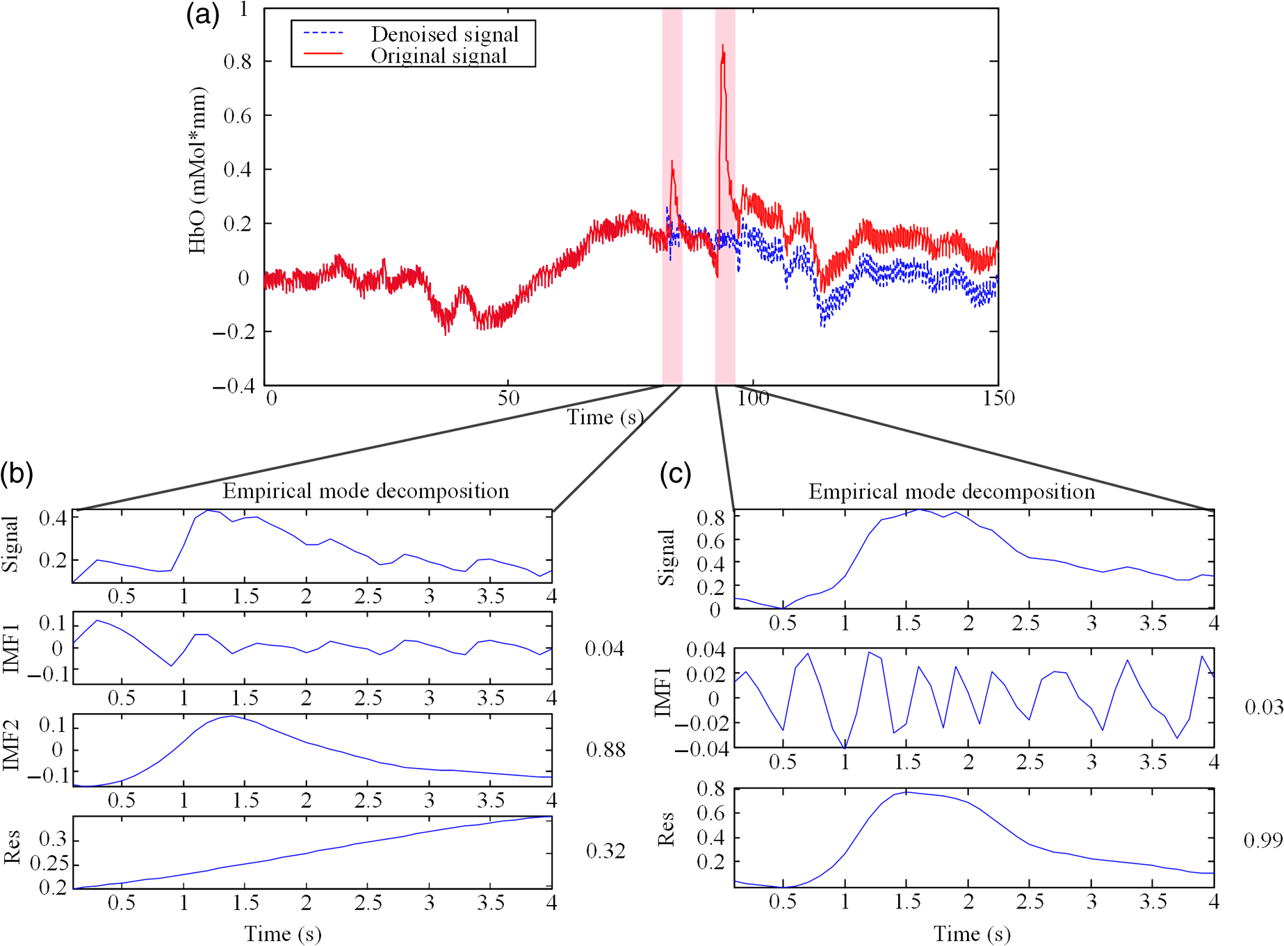

Fig. 4

(a) Synthesized HRF and (b) real resting-state data. Composite waveform obtained by adding the resting-state data to the synthesized HRF, (c) before and (d) after application of the EMD-based motion correction method.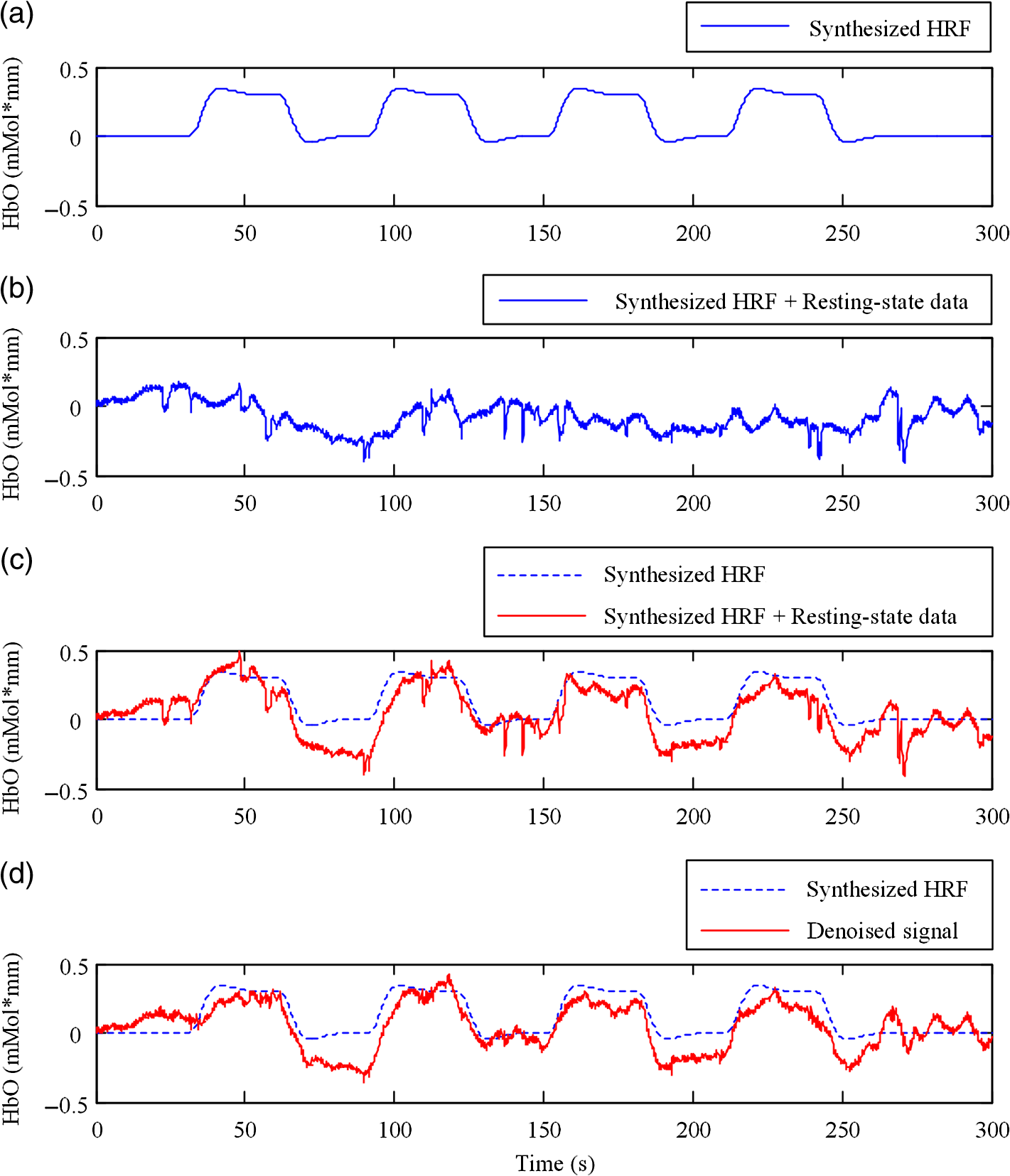

We assessed the performance of SI, kbWF, and WF for different values of their most important parameters. Figures 5(a)–5(c) show the plots of the mean MSE versus parameter value for SI, kbWF, and WF; Figs. 5(d)–5(f) show the plots of the mean SNR versus parameter value. When $p=0.99$, $k=3.4$, and $\alpha =0.04$, SI, kbWF, and WF, respectively, produced the best results. The results obtained using these parameter values were compared with the result of our proposed EMD method.

Fig. 5

(a)–(c) Average MSE obtained by SI, kbWF, and WF using different parameters; and (d)–(f) average SNR obtained by SI, kbWF, and WF using different parameters.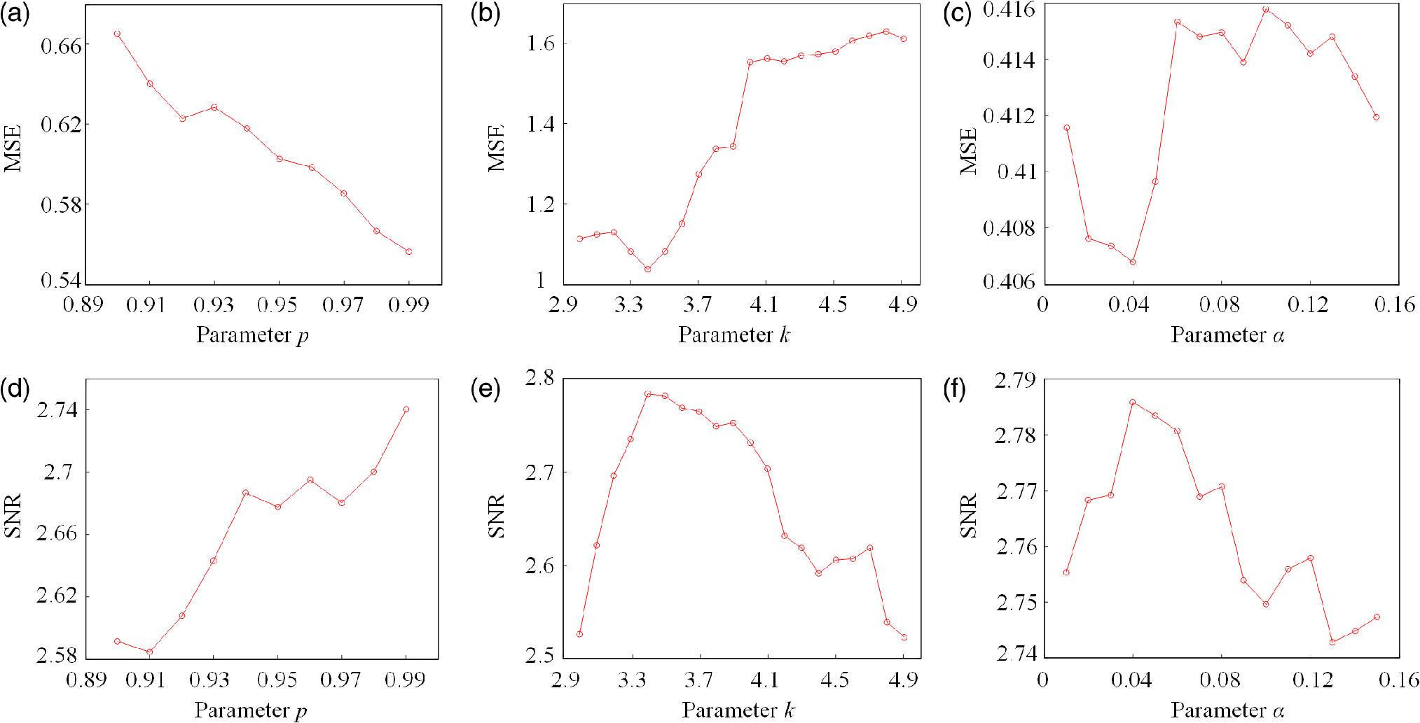

To evaluate the reliability of the methods, we analyzed the proportion of channels which were improved after applying them. The MSEs for the four methods are shown in Fig. 6, in the form of scatter plots. Each data point in the scatter plot corresponds to one fNIRS channel from one participant. The MSE before correction is the abscissa value and the MSE after correction is the ordinate value. Channels which improved in terms of MSE are below the main diagonal, whereas channels which had worse MSE after motion correction are above the main diagonal. As shown in Fig. 6(a), the EMD method reduced MSE in 79% of channels. It was more reliable than SI and WF [reduction of MSE in 75% and 73% of channels, as shown in Figs. 6(b) and 6(d), respectively] and was similar to kbWF in reliability [reduction of MSE in 80% of channels, as shown in Fig. 6(c)]. In addition, the EMD method performed consistently well at all levels of uncorrected MSE, similar to SI and kbWF, whereas WF performed badly at low levels of uncorrected MSE.

Fig. 6

Scatter plots showing the MSE of results from (a) EMD, (b) SI, (c) kbWF, and (d) WF. Each data point is a channel. Abscissa value is the MSE before correction. Ordinate value is the MSE after correction. Percentages indicate the proportion of channels above and below the main diagonal, with improved channels below the main diagonal.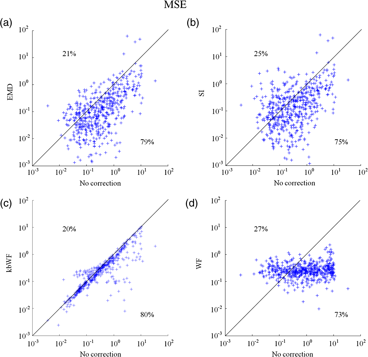

The SNRs for the four methods are shown in Fig. 7. The meanings of the abscissa and the ordinate are similar to those in Fig. 6. In this figure, channels that improved are above the main diagonal. As shown in Fig. 7(a), the EMD method performed well with an increase of SNR in 78% of channels. Only kbWF performed marginally better than the EMD method [increase of SNR in 79% of channels, as shown in Fig. 7(c)]. The other two methods were less reliable than the EMD method [increase of SNR in 73% and 72% of channels, as shown in Figs. 7(b) and 7(d), respectively].

Fig. 7

Scatter plots showing the SNR of results from (a) EMD, (b) SI, (c) kbWF, and (d) WF. Each data point is a channel. Abscissa value is the SNR before correction. Ordinate value is the SNR after correction. Percentages indicate the proportion of channels above and below the main diagonal, with improved channels above the main diagonal.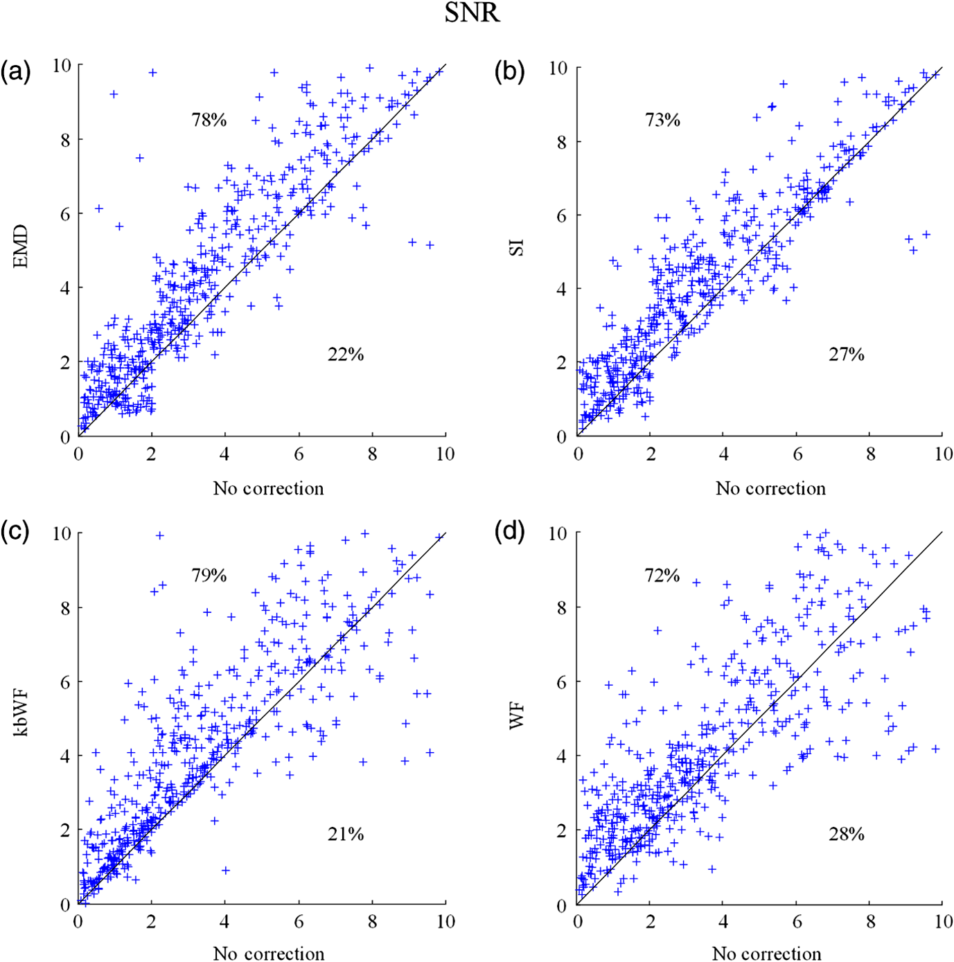

Box plots summarizing the amount of improvement across channels are shown in Fig. 8. Figure 8(a) shows the percentage change in MSE achieved by each motion correction method. EMD and SI achieved an average reduction in MSE of 53% and 51%, respectively, whereas kbWF and WF achieved an average reduction of only 23% and 35%, respectively. Figure 8(b) shows the percentage change in SNR achieved by each motion correction method. The EMD method achieved an average increase in SNR of 47%, slightly better than that achieved by SI and kbWF (42% and 43%, respectively). The WF method achieved the best average increase in SNR, 59%. Figure 8(c) shows the $R^2$ between the output of the four methods and the true signal, as well as the $R^2$ between the raw signal (no correction) and the true signal. All four methods produced an increase in $R^2$ compared with no correction ($p<0.01$, paired $t$-test). The EMD method achieved the highest average $R^2$ of 0.79, significantly higher than that of the other methods ($p<0.01$, paired $t$-test).

Fig. 8

Box plots summarizing the accuracy of each method. Each box plot shows the median, 25th, and 75th percentiles and the most extreme values not considered outliers: (a) percentage change in MSE; (b) percentage change in SNR; (c) $R^2$ between true signal and the results of EMD, SI, kbWF, and WF, as well as between true signal and uncorrected signal (no correction).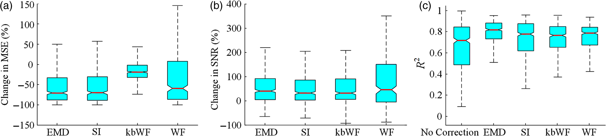

4.

Discussion and Conclusion

Motion artifacts heavily influence the quality of fNIRS recordings, especially in special populations such as infants and children. Thus, motion artifact correction is a key step in fNIRS data analysis. In the last few years, several research groups have proposed different motion correction methods to try to remove motion artifacts reliably and effectively.^{14,16,17,19,20} Although these methods perform well, they still have some limitations.^15,21 In this article, we propose a motion correction method based on EMD.

In a previous study, ensemble EMD (EEMD), an extension of EMD, was successfully used for motion artifact removal from fNIRS signals.³⁰ However, EEMD was combined with canonical correlation analysis (CCA), not used alone. Compared with a similar method (EEMD-ICA), EEMD-CCA performed better. In this study, we apply EMD alone to motion correction for fNIRS signals.

Our results indicated that the proposed EMD method was relatively reliable, produced the best or second best MSE and SNR improvements, and produced the highest $R^2$ between recovered signal and truth. The SI method also performed reliably and produced the second best percentage change in MSE, but was, overall, inferior to the EMD method. The kbWF method was slightly better than the EMD method in terms of the proportion of channels improved. However, it performed poorly in terms of the percentage change in MSE and SNR. The WF method achieved the highest percentage increase in SNR but did relatively poorly in terms of the other metrics. Overall, the proposed EMD method was the most reliable and effective motion correction method among the four.

The kbWF method is similar to the WF method, since it is a modification of the WF method. The WF method is specifically designed for spike artifacts,²⁰ but does not perform as well as the kbWF method when motion artifacts appear in many epochs and vary in size from epoch to epoch. A possible reason is that a single probability-based criterion is not sufficient to detect all motion artifacts. An iterative approach may relieve this problem; however, the iterations are difficult to be set. The kbWF method avoids this problem naturally, because it is an iterative approach which uses a kurtosis-based stopping criterion. However, because this method does not calculate the kurtosis of the first and second levels of the DWT, it is unable to detect and correct baseline shifts.

The EMD method is based on channel-by-channel artifact detection and does not assume any particular distribution of motion artifacts, similar to the SI method. In addition, it does not require any additional hardware or sensor to measure motion. An advantage of the EMD method is that it is naturally suited for use on nonstationary data, including fNIRS data. It can extract the characteristics of fNIRS data and separate the motion artifact and the hemodynamic signal more precisely than other decompositions. Thus, the performance of the EMD method is better than the other methods. Furthermore, it can correct baseline shifts. On a practical note, in order to obtain the IMFs related to motion artifacts more efficiently, we suggest retaining the high frequency information in the fNIRS signal before performing EMD. A drawback of the EMD and SI methods is that they heavily depend on accurate detection of motion artifacts. If the artifacts cannot be detected exactly, these two methods will be less accurate.

Depending on the application, the computational cost of motion correction methods may be an important consideration. We calculated the average computational times of the methods over 10 runs: EMD: $0.0539\pm 0.0005\mathrm{s}$, SI: $0.0227\pm 0.0013\mathrm{s}$, kbWF: $0.0672\pm 0.0013\mathrm{s}$, and WF: $0.0134\pm 0.0004\mathrm{s}$ ($\text{mean}\pm \text{standard deviation}$). The EMD algorithm requires repeated cubic SI to obtain upper and lower envelopes, which is computationally costly. The kbWF method is also relatively slow because it is an iterative method. However, the computational times of all four methods are acceptable when considering the time of data collection (5 min).

In conclusion, we have proposed a motion correction method based on EMD for fNIRS data. We compared our EMD method with other common motion correction methods (SI, WF, and kbWF) using real resting-state fNIRS data added to synthesized HRFs. The results showed that our EMD method is overall the most reliable and accurate method among the four. In future work, we will test whether using improved versions of EMD, such as EEMD, will result in improvements for motion artifact removal.