Deep imaging in scattering media with selective plane illumination microscopy

Adithya Kumar Pediredla; Shizheng Zhang; Ben Avants; Fan Ye; Shin Nagayama; Ziying Chen; Caleb Kemere; Jacob T. Robinson; Ashok Veeraraghavan

doi:10.1117/1.JBO.21.12.126009

20 December 2016 Deep imaging in scattering media with selective plane illumination microscopy

Adithya Kumar Pediredla, Shizheng Zhang, Ben Avants, Fan Ye, Shin Nagayama, Ziying Chen, Caleb Kemere, Jacob T. Robinson, Ashok Veeraraghavan

Author Affiliations +

Journal of Biomedical Optics, Vol. 21, Issue 12, 126009 (December 2016). https://doi.org/10.1117/1.JBO.21.12.126009

Abstract

In most biological tissues, light scattering due to small differences in refractive index limits the depth of optical imaging systems. Two-photon microscopy (2PM), which significantly reduces the scattering of the excitation light, has emerged as the most common method to image deep within scattering biological tissue. This technique, however, requires high-power pulsed lasers that are both expensive and difficult to integrate into compact portable systems. Using a combination of theoretical and experimental techniques, we show that if the excitation path length can be minimized, selective plane illumination microscopy (SPIM) can image nearly as deep as 2PM without the need for a high-powered pulsed laser. Compared to other single-photon imaging techniques like epifluorescence and confocal microscopy, SPIM can image more than twice as deep in scattering media (∼10 times the mean scattering length). These results suggest that SPIM has the potential to provide deep imaging in scattering media in situations in which 2PM systems would be too large or costly.

1. Introduction

Selective plane illumination microscopy (SPIM) is a three-dimensional (3-D) fluorescent microscopy technique in which a single planar section of the imaging volume is illuminated and imaged. Scanning plane-by-plane allows one to image the 3-D volume of interest. Figure 1 depicts the principle of operation for SPIM. Unlike confocal and multiphoton microscopy, which require point-scanning, SPIM acquires an entire image plane with a single exposure resulting in a significant reduction in the acquisition time required to image an entire 3-D volume. The technique was first introduced by Fuchs et al.¹ in 2002 to image oceanic microbes and has since become a widely used technique for applications that require a fast volumetric acquisition.

Fig. 1

SPIM experimental configuration: the excitation direction and the fluorescence detection direction are orthogonal to each other. The illumination optics is designed to create a thin light sheet at the focal plane of the imaging objective. By moving the sample in $z$ -direction, one can reconstruct a 3-D image of the sample. The right side of the figure shows images at three different depths ( $z$ ). The quality of image reduces as one image deeper from the sample surface. As a result, there is a limit beyond which the information in the image is completely lost. In this paper, we characterize both theoretically and experimentally this imaging depth limit for SPIM.

SPIM provides two significant advantages over confocal microscopy: (a) faster acquisition times due to plane scanning instead of point scanning and (b) reduced photobleaching of the sample. SPIM is shown to maintain diffraction-limited lateral resolution and high axial resolution ( $\approx 1.5 μ m$ ).² Due to the advantages mentioned above, SPIM is used extensively for in-vivo microscopy, since the fast acquisition times and reduced photobleaching allow for the imaging of dynamic phenomena. For example, Keller et al.³ and Panier et al.⁴ recorded nuclei location and movement of zebrafish using a SPIM-based multiview approach. Mertz and Kim⁵ combined the principles of light sheet microscopy and structured light to image whole mouse brain samples. Becker et al.⁶ imaged macroscopic specimens, such as mouse organs, mouse embryos, and Drosophila melanogaster. Jahr et al.⁷ used a diffractive unit to separate the spectral components of the fluorescence (from multiple fluorescence markers) to image Drosophila embryos. More recently, SPIM has been adapted for rapid volumetric imaging in the mouse cortex using a single objective lens.⁸

Here, we show that under special conditions, SPIM provides a third advantage over confocal microscopy: deeper imaging in scattering media. In instances when the excitation path length is made much shorter than the emission path length, SPIM can image twice as deep as confocal microscopy over a narrow field of view (FoV). Our findings motivate the development of implantable light emitters⁹^,¹⁰ and light guiding probes¹¹^–¹⁴ that could illuminate nearby tissue several millimeters below the surface. While miniaturized implantable SPIM probes have yet to be demonstrated, our key result shows that creating such devices would allow one to image at least twice as deep as conventional single-photon fluorescence techniques.

In the following sections, we quantitatively evaluate the depth limits for SPIM under the condition that the path lengths for excitation light and emission light are independent. For the first time, we show that under these conditions, SPIM provides a twofold improvement over confocal and epifluorescence microscopes. We also quantify how the maximum imaging depth is affected by light sheet thickness, sensor noise, and fluorophore density. Finally, we show that optimally designed SPIM systems can reach imaging depths comparable to two-photon microscopy (2PM). This deep imaging capability combined with previously demonstrated benefits of fast acquisition and low photobleaching make SPIM an attractive technique for biological imaging in scattering tissue.

2. Related Work

The depth limits of confocal and multiphoton microscopy is a well-studied property.¹⁵^–²⁰ Light scattering by tissue is the primary factor that limits the imaging depth: the stronger the scattering, the shallower the depth limit. To meaningfully account for the effect of tissue scattering while comparing the imaging capabilities of various microscopy techniques, depth limits of imaging systems are typically expressed as a multiple of the number of mean-free paths (MFPs), or scattering length, within the sample tissue.¹⁵^,¹⁷ The MFP is defined as the average distance a photon travels before a scattering event.

This definition of scattering depth limit is independent of various properties of the sample, such as density, the size of the scatterer, and wavelength. Therefore, reporting the depth in terms of MFPs provides a normalized measure to compare depth limits among various microscopic systems and tissue samples.

2.1.

Confocal Microscopy

Schmitt et al.²¹ experimentally demonstrated that the depth limits of confocal microscopy are greater than three to four MFPs using a 10-line/mm Ronchi ruling embedded in a suspension of polystyrene latex microspheres in water. Their results show that independent of the ability of the microscope to reject out-of-focus light, there exists a depth limit for confocal microscopy due to the fall of signal intensity. The depth limit is the smallest signal that can be detected by the sensor above the sensor noise floor. Schmitt et al. also showed that decreasing the diameter of the pinhole in the confocal microscope improves the rejection of background scattered light; however, the smaller pinhole comes at the cost of reduced light collection efficiency from the sample plane.

Kempe et al.²² measured the depth limit of confocal microscopy experimentally using a reflecting grating structure suspended in a solution of latex spheres and water. To simulate the effect of imaging deeper, Kempe et al. increased the concentration of the latex spheres thereby increasing the number of MFPs in their sample. When the concentration of the latex sphere was increased to 2% (in percent solid content), the contrast of the confocal microscope decreased significantly (around 50%). Based on these experiments, Kempe et al. reported an imaging depth limit of six MFPs for confocal microscope.

2.2.

Multiphoton Microscopy

In the past decade, 2PM has emerged as the most popular method for deep fluorescence imaging in scattering media due to its superior depth limit compared to confocal microscopy. Theer and Denk¹⁵^,¹⁶ were the first to analytically derive the limits for 2PM as 17 MFPs (MFP length is calculated at emission wavelength of 560 nm. In Theer and Denk’s paper, the result is reported as seven MFPs as they have calculated the MFP length at excitation wavelength.). They observed that the background fluorescence near the sample surface (i.e., excitation scattering) was the major factor limiting the imaging depth. They noted that as the imaging depth increases, the laser power at the focal point decreases due to scattering of the excitation light, approximately following the Beer–Lambertian law.²³ To compensate for this loss, one must increase the laser power as one images deeper within a scattering medium. This increased laser power results in an increase in out-of-focus fluorescence near the sample surface and thus decreases the image contrast. Hence, Theer and Denk defined the imaging depth limit as the depth at which the out-of-focus fluorescence equals the in-focus fluorescence.

As an alternative approach to estimate the depth limit of 2PM, Sergeeva²⁴ used a probabilistic model to estimate the contrast between in-focus and out-of-focus fluorescence. They reported a depth limit between 15 and 22 MFPs at which the image contrast falls to one (Sergeeva reported the depth limit as 10 to 15 MFPs, calculated at excitation wavelength, which translates from 15 to 22 MFPs at emission wavelength of 560 nm.).

Both Theer and Denk, and Sergeeva described the depth limit in terms of MFP of the excitation photons a quantity that is wavelength dependent. Because 2PM and 1PM microscopy use different excitation wavelengths we have chosen to compare the depth limits of 2PM with other imaging modalities in terms of emission MFP (Table 1). Thus, for a given fluorophore, the depth limit can be calculated based on the emission wavelength, which is independent of the method of excitation.

Table 1

Comparison of depth limits described in related works. MFP is computed for the emission wavelength, in congruence with Refs. 21 and 22.

Microscopy modality	Depth limit (as a multiple of MFP)	Reference
Confocal	3 to 4	21
Confocal	6	22
2PM	17	16
2PM	15 to 22	24

2.3.

Selective Plane Illumination Microscopy

Despite the growing popularity of SPIM, the fundamental imaging depth limit of this microscopy technique has yet to be characterized either theoretically or experimentally. Recently, Glaser et al.²⁵ utilized Monte Carlo simulations to compare the signal to background ratio of SPIM with the dual axis confocal microscopy. Paluch et al.²⁶ reported that in their experiments, the signal strength and the noise strength of SPIM are equal at 10 MFPs but did not characterize the factors that affect this maximum imaging depth. Here, using the openSPIM system,²⁷ we also show a depth limit close to 10 MFPs and take this result further to identify the major factors that influence this imaging depth.

To computationally estimate the maximum imaging depth for SPIM, we employ a Monte Carlo sampling-based approach and compare these results to measured data. We also compare the depth limits of SPIM with confocal, epifluorescence, and 2PMs for brain phantoms and fixed brain tissues. For the first time, our results show that SPIM can image almost twice as deep as confocal microscopy. We also demonstrate that by optimizing the imaging conditions for SPIM, we can approach the imaging depth of 2PM (15 MFPs compared to 17 MFPs). The fact that SPIM has significantly faster acquisition rates compared to point scanning methods, limited photobleaching, and deep imaging capabilities, suggests that SPIM should be considered a practical alternative to conventional microscopy techniques in scattering media.

2.4.

Two-Photon Microscopy-Selective Plane Illumination Microscopy

Palero et al.²⁸ proposed to combine the advantages of 2PM microscope and SPIM, and designed a 2PM-SPIM. The effective light sheet thickness of the 2PM-SPIM is smaller compared to the 1PM-SPIM discussed in this paper. (For the brevity in notation, we have referred 1PM-SPIM as SPIM in the entire paper, unless we are comparing 1PM-SPIM and 2PM-SPIM.) Hence, 2PM-SPIM can image deeper than the 1PM-SPIM, which is also reported by Truong et al.²⁹ Also, the excitation scattering is lower in 2PM-SPIM compared to the 1PM-SPIM. As a result, the light sheet will remain thin over a long propagation length compared to 1PM-SPIM, resulting in larger FoVs deep in scattering media. Though the depth limits of the 1PM-SPIM and 2PM-SPIM are different, the fundamental model proposed in this paper can be extended to 2PM-SPIM, but the exact characterization of the depth limit is beyond the scope of this paper.

3. Problem Statement

Scattering of light is the primary factor limiting the imaging depth of most optical microscopes. For fluorescence imaging techniques such as SPIM, scattering can be classified into two types: excitation scattering and emission scattering. “Excitation scattering” is defined as the scattering of source photons, while “emission scattering” is defined as scattering of fluorescently emitted photons that have a longer wavelength than the source photons. Excitation scattering can also cause “secondary fluorescence,” as depicted in Fig. 2. Scattered excitation photons can excite unintended fluorophores that then emit light at the emission wavelength.

Fig. 2

Monte Carlo simulations: the photons from light sheet that excite the fluorophores are called excitation photons. Some of these excitation photons are scattered and cause secondary fluorescence. The fluorescent molecules that are excited emit photons, referred to as emission photons. Some emission photons reach the objective without getting scattered, referred to as ballistic photons. Some emission photons reach the objective after single or multiple scattering events, referred to as scattered photons. Some emission photons get scattered outside the FoV of the imaging system.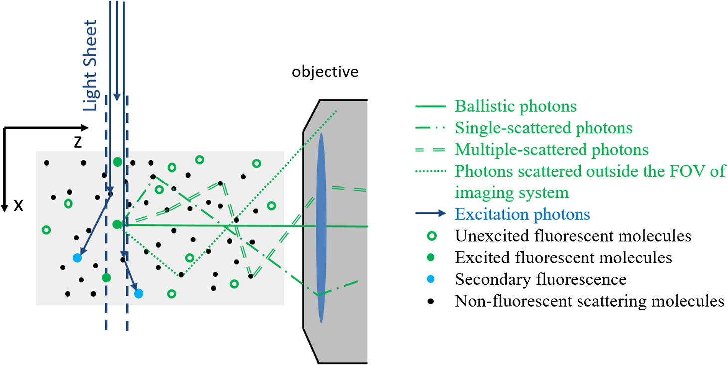

Some of these emission photons, referred to as ballistic photons, reach the detector without getting scattered at all. However, many emission photons are either scattered once or more before reaching the imaging system. Because excitation and emission photons are generated by different sources, we treat them separately. For SPIM, excitation scattering is independent of the imaging depth because excitation light travels orthogonal to the imaging axis. In other words, at each depth, the excitation light travels the same distance from the source. Excitation scattering results in unwanted background fluorescence, the strength of which can be decreased by decreasing the light sheet thickness. However, the minimum sheet thickness is determined by the diffraction limit of the excitation light. Emission scattering, on the other hand, does depend on the imaging depth.

Informally, we define the depth limit as the depth below which we cannot distinguish between the signal coming from a specific fluorophore and the signal coming from other sources, such as emission scattered light, secondary fluorescence, and sensor noise. The signal measured by the sensor is influenced by multiple factors including photons arriving from the fluorophore of interest (we will call them photon flux), denoted by ( $P$ ), photons arriving from the background ( $B$ ) due to scattering, Poisson noise of the photon flux and background, quantum efficiency of the sensor ( $Q_{e}$ ), exposure duration ( $t$ ), sensor read noise ( $N_{t}$ ), and dark current ( $D$ ). It is easy to robustly estimate the average background signal.³⁰^,³¹ Hence, we can subtract the background from the measured signal. However, the variance in the background caused by the Poisson noise cannot be removed. Hence, we define signal-to-noise ratio (SNR) as follows:

Eq. (1)

SNR = \frac{P Q_{e} t}{\sqrt{((P + B) Q_{e} t + D t + N_{t}^{2})}},

in line with the definition in Ref. 32. Formally, we define depth limit as the depth at which the signal power and the noise power are equal, alternatively, the depth below which the SNR falls below unity. Note that the SNR is a function of light sheet thickness, fluorophore density, and photon emission rate. In this work, we characterize the depth limit as a function of these parameters and since many of these parameters have fundamental depth limits themselves, this allows us to estimate the fundamental depth limit for the ideal SPIM microscopes. Note that one could improve the accuracy of our model for SNR by considering the spherical aberrations of the lens; however, for the lens we have used in our experiments, the spherical aberrations are negligible and we therefore neglect the effect of spherical aberrations in our theory.

3.1.

Assumptions

We assume a homogenous distribution of scattering particles and fluorophores in the sample. We also assume that the light sheet does not have shadows cast by scattering particles, which could reduce the maximum depth limit.

4. Computational Model to Characterize Depth Limit

To characterize the depth limit, we first calculate the fluorophore bead intensity as a function of depth. The depth limit will be the depth at which this signal is equal to the total variance created by various sources (Poisson noise, sensor noise, and so on), which we refer to as the visibility threshold. To predict the fluorophore intensity, we employ the classical radiative transfer equation (RTE)³³^–³⁵ given in the standard integrodifferential equation for plane-parallel medium as follows:

Eq. (2)

\cos θ \frac{d I (θ, φ)}{d z} = - σ_{ext} I (θ, φ) + \frac{σ_{sca}}{4 π} \int_{θ^{'} = 0}^{2 π} \int_{φ^{'} = 0}^{π} \sin θ^{'} p (θ^{'}, φ^{'}, θ, φ) d θ^{'} d φ^{'},

where

θ

and

φ

are the azimuth and elevation angles,

I

is the intensity at depth

z

,

σ_{ext}

and

σ_{sca}

are the extinction and scattering cross-sections of the scattering particles and

σ_{ext} = σ_{sca}

for purely scattering medium,

p (\cdot)

is the probability (or percentage) of incident radiation traveling in the

(θ^{'}, φ^{'})

direction that will shift to

(θ, φ)

direction upon scattering. The first term in the RTE models the amount of light lost due to extinction (absorption + scattering), whereas the second term models the amount of light gained due to scattering in the neighborhood.

While the exact solution to the RTE has yet to be reported, multiple approaches³⁶^,³⁷ to find approximate solutions for the RTE are available in the literature. In this paper, we approximate a solution to Eq. (2) using a Monte Carlo model described below, where photon transport from each fluorophore is computed using graphics inspired techniques.

4.1.

Monte Carlo Model to Solve Radiative Transfer Equation

To render the fluorophore, we track many virtual photons emitted by the fluorophore as they pass through the scattering media (see Fig. 2). To track each photon, we model the samples as a random process. For a given scattering particle, photon arrival can be modeled as a Poisson process. We can change our frame of reference such that we model a stationary photon with scattering particles arriving according to a Poisson process. The interarrival time for a Poisson process is geometrically distributed.³⁸ In this case, the arrival time manifests as the distance between two scattering events of the photon. Hence, the distance traveled by the photon before hitting a random scatterer is given by $d = - d_{s} \log ξ$ , where $d_{s}$ is the MFP length and $ξ \sim U [0, 1]$ . After a photon hits a scattering particle, the propagation direction of the photon can change. This deviation is dependent on the scattering medium and manifests as the $p (\cdot)$ term in the RTE [Eq. (2)]. We model this deviation using Henyey–Greenstein probability density function,³⁹ which is given by

Eq. (3)

\cos θ = \frac{1 + g^{2}}{2 g} - \frac{{(1 - g^{2})}^{2}}{2 g (1 - g + 2 g ξ)},

where

g

is the anisotropic parameter and is around 0.9 for brain tissue.⁴⁰ The azimuth after scattering is uniformly distributed. After scattering, the directional cosines of the deflected ray will be altered. We employed the electric field vector, the magnetic field vector, and the direction of the photon as the basis for the 3-D space and used the fact that the direction of the electric field before scattering, the direction of the electric field after scattering, and the direction of scattered photon are coplanar⁴¹ to find the basis after each scattering event. This approach to track the photon and polarization vectors was first proposed by Peplow.⁴² After the photons exit the sample, they are focused to the sensor through lenses in a

4 f

system. We made the thin lens approximation to model the lens system and track the photon until it reaches the sensor.

The Monte Carlo simulation model that we have proposed in this paper is comparable to the models by Blanca and Saloma⁴³ for 2PM, and Schmitt et al.²¹^,⁴⁴ for confocal microscopy. Our Monte Carlo code along with the other scripts and data are made available online.⁴⁵ Though we consider polarization of the photons, it has to be noted that our Monte Carlo method does not model interference. However, the light emitted by the fluorophore has a typical coherence length of only a few microns⁴⁶ and thus, the interference effects can be safely neglected at the imaging scales of interest.

4.2.

Results and Derivation of the Theoretical Depth Limit

Using the Monte Carlo method, we first estimated the observed intensity (in a SPIM microscope) of fluorophore beads located at various depths in the scattering tissue. The resulting curve is shown in Fig. 3. We also experimentally verified the data by imaging fluorescent polystyrene microspheres suspended in a matrix of nonfluorescent microspheres with the approximate scattering properties of brain tissue (i.e., brain phantom, see Sec. 6). Since the intensity of fluorophores we measure is a function of exposure duration, we cannot directly compare the experimental fluorophore intensities with the simulation results. Hence, we normalize both experimental and Monte Carlo simulation results to have unit intensity at the sample surface, which corresponds to an imaging depth of less than one MFP. From Fig. 3, we observe that the experimental fluorophore bead intensities at various imaging depths are close to the intensities predicted using our model. We have experimentally measured the visibility threshold near the depth limit for a Hamamatsu sensor (type number: C4742-95-12ER). Recall that the theoretical depth limit is the depth at which the Monte Carlo predicted bead intensities fall below this visibility threshold. Using the values from the Monte Carlo simulation (Fig. 3), we can conclude that the theoretical depth limit is between 9 and 11 MFPs.

Fig. 3

Monte Carlo model and predicted depth limit: simulated (blue line) and experimental (black dot) intensity decay curves for fluorophores imaged with SPIM. We normalize both experimental and Monte Carlo simulated results to have unit intensity at the surface region of the tissue corresponding to an imaging depth of zero to one MFP. Around 9 to 11 MFPs, the predicted intensity of the fluorophore goes below the visibility threshold (dashed red line), which is equivalent to a SNR of 1. Hence, 9 to 11 MFPs is the theoretical and experimental depth limit of the open SPIM used for our analysis.

It should be noted that this particular method for finding the depth limit is informed by experimental results that set the visibility threshold. The background variance part of the visibility threshold is dependent on vortex mixing during the sample preparation, preventing us from calculating the visibility threshold. However, once we know the visibility threshold for a particular SPIM system, we can predict this threshold for other SPIM systems by scaling the threshold appropriately (according to physical parameters of the system, such as light sheet thickness, fluorophore density, sensor characteristics, and so on). In Sec. 4.3, we investigate how the light sheet thickness and sensor properties affect the depth limit for SPIM.

4.3.

Depth Limit Characterization

The depth limits of a particular SPIM system are primarily determined by the light-sheet thickness and sensor noise level. Therefore, we characterize the depth limit as a function of light sheet thickness and sensor noise. As the light sheet thickness increases, the amount of background fluorophore light increases linearly. Therefore, an increase in light sheet thickness results in an increase in the variance of the background and thereby contributes to an increase in the visibility threshold. The increase in visibility threshold decreases the depth limit of imaging according to the graph shown in Fig. 3. Increasing the fluorophore density has a similar effect as increasing the light sheet thickness.

When we use a sensor with lower noise characteristics, it is natural to expect that the imaging depth limit would increase. Formally, this effect appears in Eq. (2) as a decrease in the visibility threshold as the sensor noise is reduced. Similarly, an increase in fluorophore emission rate is also expected to increase the imaging depth limit as each fluorophore will emit more photons, increasing the signal intensity. Assuming that the fluorophore emission rate has increased by a factor of $κ$ ( $κ > 1$ ), both the photon flux and the background flux are increased by the same factor of $κ$ . The new SNR increases approximately by a factor of $\sqrt{κ}$ and is given by

Eq. (4)

SNR = \sqrt{κ} \frac{P Q_{e} t}{\sqrt{(P + B) Q_{e} t + \frac{D t + N_{t}^{2}}{κ}}} .

The increase in SNR will result in a corresponding increase in the depth limit of the SPIM.

To calculate the imaging depth limit for a general SPIM system, we can scale the background variance according to the light sheet thickness, and we can adjust the sensor noise characteristics. By rescaling Fig. 3 in this way, we compute the depth limit for arbitrary sheet thicknesses and sensor performance. We plot this result in Fig. 4, which shows the expected depth limit for various light sheet thicknesses and sensor noise levels. We notice that as the light sheet thickness or the sensor noise levels increases, the depth limit decreases. It should also be noted that this depth limit graph is valid only if other parameters like the field-of-view, fluorophore density, and fluorophore emission rate are held constant. To make this fact more explicit, we rewrite the light sheet thickness more generally as the number of background photons per second and add this axis to the top of Fig. 4. The background photon rate is calculated as the product of the field-of-view of a pixel in the sensor ( $1 μ m \times 1 μ m$ ), light sheet thickness, fluorophore concentration (61 million molecules/ml), and fluorophore emission rate (2 million photons/molecule/second).⁴⁷

Fig. 4

Characterization of depth limit: (a) Depth limit as a function of light sheet thickness and sensor noise. The axis label Average background represents the average number of background photons per second for our SPIM system. This value is obtained by multiplying the light sheet thickness with the FoV of a pixel ( $1 μ m \times 1 μ m$ ), fluorophore concentration (61 million molecules/ml), and fluorophore emission rate (2 million photons/molecule/s).⁴⁷ (b) Predicted depth limit for different commercially available sensors for various light sheet thicknesses. Independent of the sensor, as the light sheet thickness decreases, we observe an increase in the depth limit. (c) Predicted depth limit for various sensor noise levels at a given light sheet thickness. We observe a decrease in the depth limit as the sensor noise increases.

4.4.

Validation of Depth Limit Characterization

To verify the predicted dependence of the depth limit on light sheet thickness, we analyzed the imaging depth as a function of the distance from illumination source. We chose this experiment because the incoming light-sheet illumination expands as the light propagates through sample. Thus, the light sheet thickness expands uniformly as a distance from the source giving us the ability to test our model using the natural expansion of the light sheet without physically altering the experimental setup. Moreover, this kind of validation also enables us to understand the effect of imaging farther from the excitation source ( $x$ -direction in Fig. 1).

To estimate the light sheet thickness at a distance $x$ from the illumination source, we used Monte Carlo simulations. The photons are initialized on a thin light sheet and are uniformly distributed along $y$ -axis direction and Gaussian distributed along $z$ -axis direction with full-width-half-maxima (FWHM) equal to the light sheet thickness of our SPIM system ( $\sim 7 μ m$ ). To generate the initial $z$ -coordinate for photons, we used a Box–Muller transformation.⁴⁸ The sensor (virtual) is placed parallel to $y z$ -plane at a distance $x$ . After computing the light sheet thickness, we queried the depth limit characterization plot to estimate the depth limit as a function of the distance from the light source and plotted Fig. 5. The blue curve shows the estimated depth limit as a function of the distance from the light source. We plotted the empirically measured values in red. We observe that the estimated depth limits follow our experimental results with a maximum deviation of 1 MFP confirming our calculations for how the maximum SPIM imaging depth depends on light sheet thickness.

Fig. 5

Validation of depth limit characterization. We compute the light sheet thickness as a function of distance ( $z$ -direction) from the light source using Monte Carlo simulations. Using the depth-limit characterization graphs, we compute the corresponding depth limit as a function of distance from the source, which is represented by the blue curve. We have also measured the depth limit experimentally and plot this limit as red crosses. Notice that the depth limits estimated by our technique and the observed depth limits match with a maximum error of 1 MFP.

4.5.

Depth Limit of Two-Photon Microscopy-Selective Plane Illumination Microscopy

Recall that the 2PM-SPIM suffers from less excitation scattering compared to the 1PM-SPIM²⁸ producing a thinner light sheet in scattering media. Hence, based on the discussion we have in Secs. 4.3 and 4.4, 2PM-SPIM can image deeper than the 1PM-SPIM, which is also reported by Truong et al.²⁹ Also, because the light sheet will remain thin for longer propagation lengths, 2PM-SPIM can produce larger FoVs deep within scattering media. Though the depth limits of the 1PM-SPIM and 2PM-SPIM are different, the fundamental model proposed in this paper can be extended to 2PM-SPIM, but the exact characterization of the depth limit is beyond the scope of this paper.

5. Comparisons of Depth Limits with Epifluorescence, Confocal, and Two-Photon Miroscopy Microscopes

Epifluorescence, confocal, and 2PM microscopes are the most common volumetric microscopy techniques. In this section, we compare the depth limits of SPIM with these common imaging modalities. To perform this comparison, we prepared a series of brain phantoms and fixed brain tissue, and imaged these samples using the aforementioned four microscopes: an epifluorescence microscope, a confocal microscope, a SPIM microscope, and a 2PM. Section 6 describes the preparation of samples and the procedures used to image them. In this section, we compare the results.

5.1.

Comparison of Depth Limits of Various Microscopy Techniques on Brain Phantoms

To compare 3-D microscopy techniques, we prepared a tissue phantom with the approximate scattering properties of the brain using a suspension of fluorescent and nonfluorescent polystyrene microspheres (see Sec. 6). Figure 6(a) shows $x$ – $y$ images of individual beads captured at different depths using each of the microscopy techniques. Notice that the depth limits of epifluorescence and confocal microscopes are less than five MFPs, whereas SPIM can image between 9 and 11 MFPs. We repeated the experiment on multiple samples and with brain phantoms of different densities. Table 2 summarizes the depth limits of various brain phantoms. We can observe that the ratio of the depth limit to MFP length, which we expect be a constant, is slightly lower for larger MFP length. This decrease in the depth limit for large MFPs has also been observed in 2PM.¹⁷ For long MFPs, the total distance traveled by the emitted photons is greater, thus we expect that other loss mechanisms like absorption may contribute to lower, shallower than expected depth limits.

Table 2

Experimental depth limits of SPIM for various brain phantoms.

Density compared to brain phantom	MFP	Depth limit (μm)	Depth limit average (#MFPs)
100%	75.03	807.89	10.64
50%	140.12	1422.21	10.15
25%	238.53	2199.24	9.33

Fig. 6

SPIM versus other microscopies for brain phantom. (a) $y$ – $z$ maximum intensity projection of the 3-D volume of brain phantom as imaged by epifluorescence microscopy, confocal microscopy ( $ν = 50$ optical units), confocal microscopy ( $ν = 1.3$ optical units), SPIM, and two-photon microscope. (b) The number of visible beads per square millimeter at each depth for the five different microscopy methods. (c) Cropped $x$ – $y$ images of individual beads at various imaging depths from each of the microscopy techniques. Images are zoomed-in ( $4 \times$ ) for each bead. All $x$ – $y$ slice images show both postprocessed images with adaptive histogram equalization to improve the visual quality (left) and raw data (right).

Figure 6 also shows a $y$ – $z$ projection of the images collected from the brain phantom using an epifluorescence microscope, a confocal microscope (pinhole sizes of 1.3 and 50 optical units), a SPIM and a 2PM. We also counted the number of visible beads per image frame and plotted this number as a function of imaging depth (averaged over four samples). We observe that at the surface region of the phantom, the bead counts of all imaging modalities are almost the same. However, the bead count quickly drops as we image deeper using epifluorescence and confocal microscopy. Epifluorescence imaging appears to have slightly more visible beads because this method can observe more out-of-focus beads than any of the other imaging techniques. Hence, even though epifluorescence imaging shows more beads, they are not necessarily located at the depth of the focal plane. As expected, confocal microscopy with an optimized pinhole size (1.3 optical units) has better depth resolution than confocal microscopy with a large pinhole size (50 optical units). Thus, the depth limit of confocal microscopy with the optimized pinhole size is higher than the confocal microscopy with large pinhole size. However, both methods show depth limits between three and four MFPs. SPIM has a depth limit of 9 to 11 MFPs, which is two to three times deeper than other single-photon microscopy modalities. The 2PM can image even deeper than SPIM, most likely due to the fact that 2PM can better confine the excitation volume and thus reduce the background fluorescence. Due to the limited working distance of our 2PM, we can explore a maximum depth of around $1160 μ m$ (15.52 MFPs) before the objective lens contacts the sample surface. At this maximum depth, determined by the working distance of the objective lens, the beads have very low intensity. Thus, we predict that the imaging depth limit is slightly longer than 15.52 MFPs. We repeated the experiment on multiple samples and summarized the results in Table 3.

Table 3

Depth limit comparison of various imaging modalities for brain phantom.

Imaging modality	Depth limit (μm)	Depth limit average (#MFPs)
Epifluorescence	255.10	3.40
Confocal ( $ν = 50$ )	297.87	3.97
Confocal ( $ν = 1.3$ )	335.38	4.47
SPIM	799.32	10.64
2PM	$> 1164$	$> 15.51$

The factors that limit the maximum imaging depth are different for each imaging modality. Epifluorescence imaging suffers from both excitation scattering and emission scattering, and thus, the images appear less sharp with bright background levels. Confocal imaging blocks most emission scattering but still suffers from excitation scattering. Additionally, near the depth limit, the confocal system has very little light that reaches the sensor through the pin hole. Thus, the count noise on the image sensor becomes a significant factor that limits the imaging depth. SPIM effectively eliminates most of the effects of excitation scattering. Because this method suffers primarily from emission scattering alone, it has a much deeper maximum imaging depth compared to other single-photon excitation microscopy techniques. In these samples, the depth limit of SPIM is likely limited by the finite sheet thickness, which does not confine the excitation volume as well as 2PM. We expect that in the limit of a diffraction-limited light sheet, 2PM and SPIM would have the same depth limit ( $\sim 15 MFPs$ ), as shown Fig. 4(a).

5.2.

Comparison of Depth Limits of Various Microscopy Techniques on Brain Tissue

We also compared the depth limits of the major 3-D fluorescent microscopy techniques using a fixed brain tissue sample isolated from the cerebral cortex of a mature male Long–Evans rat. After performing perfusion and fixation by paraformaldehyde (4% PFA in buffer), the sample becomes denser than live brain tissue. Then, it is stained in diluted NeuroTrace 500/525 green fluorescent Nissl stain. Note that the fixation process greatly increases the amount of light scattering in the tissue sample leading to a MFP that is reduced by roughly a factor of 2 compared to live tissue. Figure 7 shows both the $x$ – $y$ view at different depths and the $y$ – $z$ view of the cerebral cortex as imaged by the epifluorescence microscope, confocal microscope ( $ν = 50$ optical units), confocal microscopy ( $ν = 1.3$ optical units), SPIM, and a 2PM. In the $x$ – $y$ slice, we can notice neurons as bright ellipses. We postprocessed the $x$ – $y$ slices with an adaptive histogram equalization method to improve the visual quality of the slices. The behavior of signal intensity with respect to background as we image deeper is similar to that of a brain phantom. We also counted the number of visible neurons per image frame and plotted the decay curve of visible neurons per image as a function of imaging depth. One difference from the brain phantom’s decay curve is that the decay curve is relatively flat at mid depths and then drops suddenly at large depths. This phenomenon is likely due to the fact that a $1 - μ m$ bead in the brain phantom occupies only a few pixels and is difficult to identify as it blurs. However, for brain tissue, a $10 - μ m$ neuron occupies many pixels and can therefore be identified upon blurring. This phenomenon also accounts for a smoother variation in distinguishable neurons compared to the number of beads visible in the brain phantom (Fig. 6). Based on these measurements, we identified the depth limits of the epifluorescence, confocal, SPIM, and 2PMs for fixed brain tissue samples as 2.50, 3.38, 3.85, 8.92, and 17.53 MFPs, respectively, which are similar to results of the experiments in the brain phantom. As described in Sec. 4.5, the 1P-SPIM depth limits can be improved by using a multiphoton light-sheet.

Fig. 7

SPIM versus other microscopies for fixed brain tissue. (a) $y$ – $z$ view slices of the fluorescence distribution in a subvolume of brain tissue by epifluorescence microscopy, confocal microscopy ( $ν = 50$ optical units), confocal microscopy ( $ν = 1.3$ optical units), SPIM and two photon microscope. (b) Plot shows the corresponding decay curves of the number of visible neurons per 1 square millimeter on camera frame. (c) Cropped $x$ – $y$ view images of camera frame at various imaging depths in different modalities. All $x$ – $y$ slice images are postprocessed with adaptive histogram equalization to improve the visual quality, as shown on the right side of the raw images.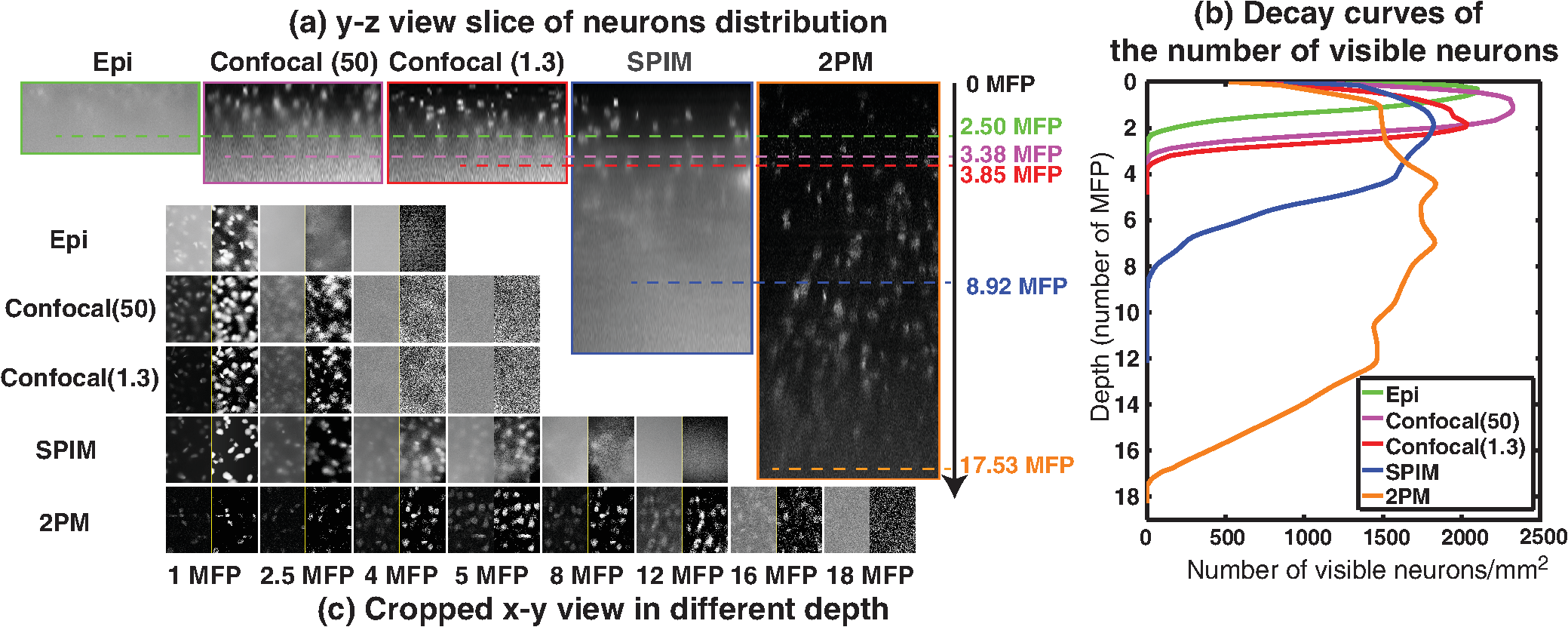

5.3.

Comparison of Depth Limits of Various Microscopy Techniques Using Contrast-Based Metric

The depth limits derived and characterized in this paper are based on the detection of point sources like fluorescent beads or neurons. Depending on the imaging application, other metrics to describe the depth limit may be more appropriate. For example, an alternative metric to determine the maximum imaging depth has been defined previously as “useful contrast.”²⁹ In this section, we compare our results to the depth limits predicted by the “useful contrast” metric.

The useful contrast at various depths has two components: the $x$ -component and the $y$ -component. The $x$ -component of useful contrast is defined as the ratio of the spectral energy of the signal corresponding to $x$ -direction-spatial-wavelength of 2.5 to $20 μ m$ , to the total spectral energy of the image. The $y$ -component is defined similarly with $y$ -direction-spatial wavelengths. Hence, for a flat image with no identifiable structures, useful contrast in both directions is unity. In practice, however, we were unable to identify any structures at values slightly higher than unity. Thus, the detection threshold using the useful contrast metric is an empirical value $> 1$ .

Figures 8(a) and 8(b) show the useful contrast fall-off for $x$ and $y$ directions for confocal, SPIM, and 2PM microscopes. We also have marked the depth limits as computed by the detection-metric we have used in this paper. We can observe that except for the $x$ -component of useful contrast of SPIM, the useful contrast is nearly the same (1.75) for all the imaging modalities [confocal (1.3), SPIM and 2PM]. Thus, for our samples, 1.75 represents the empirical useful contrast value at the depth limit. Unfortunately, while the useful contrast metric is utilitarian when imaging tissue specimens, phantom experiments are not suitable for this metric. This is because the number of beads in the sample varies rapidly with depth because the beads are randomly distributed throughout the tissue phantom. Unfortunately, useful contrast as a metric is quite sensitive to the number of beads in the sample (especially when the number of beads is small). The result is large variations in the useful contrast metric that are not representative of the actual imaging contrast. We have also excluded the epifluorescence and confocal (50) graphs in the comparison, as these plots are very close to the confocal (1.3) plots and are decreasing the readability of the figure. For applications that require greater image contrast, the depth limits will likely be reduced indicating that the metric employed in this paper is close to the upper bound for imaging depth.

Fig. 8

Comparison of depth limits derived with detection metric to “useful contrast” proposed by Truong et al.²⁹ (a) $x$ -component and (b) $y$ -component of useful contrast. The dotted vertical lines indicate the depth limits determined using the detection metric and the horizontal line indicates the threshold, where the detection metric and the “useful contrast” metric exhibit similar behavior. The $x$ -component of the detection metric for SPIM is slightly higher due to the spectral component introduced by the illumination fall off.

6. Methods

Here, we describe the experimental methods for preparing a brain phantom and brain tissue as well as the procedure used to measure the MFP. We will also give details of various steps involved in imaging these samples with confocal, epifluorescence, two-photon, and SPIM microscopes.

6.1.

Preparation of Samples

In this section, we give comprehensive details employed for the preparation of various samples that can help researchers in replicating the samples for imaging.

6.1.1.

Preparation of brain phantom

To prepare a brain phantom for imaging, we suspend blue–green fluorescent ( $1 - μ m$ diameter, 488/560) and nonfluorescent polystyrene beads ( $1 - μ m$ diameter) in agar/milli-Q solution. Low melting agar powder is measured out to be 1% wt/v of the final sample volume and added to the milli-Q water. The milli-Q water is heated to boiling to activate the agar. Then, the milli-Q/agar solution is vortexed (spun on a vortex spinner) to make agar evenly mixed up. Next, we add fluorescent and nonfluorescent polystyrene beads into the milli-Q/agar solution. Fluorescent and nonfluorescent beads are stored separately in a suspension, which has beads per mL. The proportion of milli-Q water to sample suspension is calculated based on the initial bead suspension concentration and the target concentration of the sample. The beads cannot be heated above 97°C, so the milli-Q/agar solution is cooled down from 60 to 85°C before the beads are added. After adding the beads, the sample is vortexed to ensure that the beads are evenly distributed in sample suspension before it is transferred into syringes and cuvettes. These containers are refrigerated for several minutes to make the sample coagulated. We made sure that the samples across various experiments like measuring MFP, computing experimental depth limits of SPIM, and other imaging modalities come from the same batch. For the brain phantom, in the final sample volume, we have about $5.46 \times 10^{9}$ nonfluorescent beads per mL as scatterers to simulate brain tissue and about $10^{6}$ fluorescent beads per mL as features to measure depth limit.

6.1.2.

Preparation of brain tissue

To prepare brain tissue for imaging, we fixed and extracted the brain of an adult Long Evans rat and stained neurons with a green fluorescent dye. (The sample was obtained from animals euthanized as a result of other procedures approved by the Institutional Animal Care and Use Committee at Rice University conforming to National Institutes of Health guidelines.) The animal was transcardially perfused with 4% PFA in phosphate-buffered saline (PBS) solution. After further fixation, the brain was manually divided into $\sim 1 - mm$ coronal sections using a brain slicer matrix. Sections were incubated for 24 h at 4°C in a solution containing a NeuroTrace 500/525 fluorescent Nissl stain (Molecular Probes, 1:200 dilutions in 0.1M PBS). The stained sections were then cut into $\sim 1 mm$ strips along the horizontal plane and divided at the midline, with samples from either hemisphere paired for SPIM and control imaging purposes. Samples $\sim 3 mm$ from the dorsal cortical surface were imaged by suspending them in agar in a syringe tube (SPIM) or mounting them on a microscope slide and sealing with agar (epifluorescence, confocal, and two-photon).

6.2.

Measuring Mean-Free Path for Brain Phantom

We first compute MFP using Mie scattering theory. Later, we experimentally calculate the MFP and verify that the experimentally verified value is close to the theory. The MFP length of the sample is given by⁴⁹

Eq. (5)

MFP = \frac{2 d}{3 φ Q_{s}},

where

d

is the mean diameter of the bead,

Q

is the scattering efficiency factor (wavelength dependent), and

φ

is the volume density of the scattering medium.

In the brain phantom sample we have used, we have $5.46 \times 10^{9}$ beads per mL and the average diameter of the bead is $1 μ m$ . The scattering efficiency of polystyrene at 632.8 nm is 2.7784.⁵⁰ Hence, using Eq. (6), the MFP for the brain phantom is calculated to be $83.91 μ m$ at 632.8 nm or $74.25 μ m$ at 560 nm. The MFP for the half and quarter concentration brain phantoms used in our experiments is 148.50 and $297.00 μ m$ .

However, as the preparation of phantom is not very reliable and is subject to procedural errors, such as wrong concentration of beads that may have perturbed the MFP of the sample, the actual MFP of the phantom can deviate from the calculations of the Mie theory. Therefore, we experimentally measured the MFP of each phantom sample employed in our experiments and used this experimentally measured MFP for normalizing the depth limits.

Figure 9(a) shows the side view of laser scattering from the sample. The vertical profile of the image for various column pixels is shown in Fig. 9(b). Let $I (d)$ be the intensity profile of a vertical plane, $τ$ be the MFP, and $d_{s}$ be the starting location of the beam. If we employ the zeroth order approximation of RTE, we get Beer–Lambertian law²³ and we have

Eq. (6)

I (d) = α \exp (- \frac{d - d_{0}}{τ}),

where

d > d_{0}

is the depth.

α

accounts for the intensity of the laser, quantum yield, and albedo. Taking logarithm on both sides, Eq. (6) becomes

Eq. (7)

\log I (d) = \log α - \frac{d}{τ} + \frac{d_{0}}{τ} .

Fig. 9

Experimental data to measure MFP. (a) The laser beam is scattered as it goes through the medium (brain phantom). (b) For a length up to single scattering event, the laser intensity profile is going to decrease logarithmically with decay rate of 1/MFP. By measuring the rate of decay of the beam for various columns, we estimate the MFP length of the sample.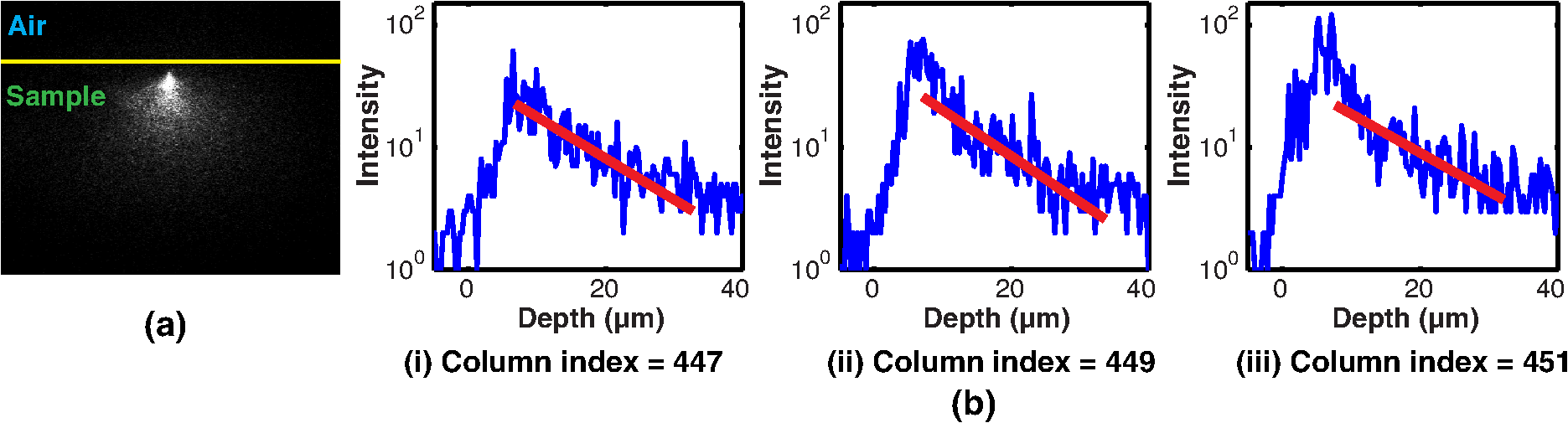

Hence, the slope of $\log I (d)$ versus $d$ plot gives us $- \frac{1}{τ}$ and is independent of both $α$ and $d_{0}$ . Therefore, we fit a straight line for the log measurements, as shown in Fig. 9(b).

There are multiple column pixels in Fig. 9. Naturally, the average of the MFPs of all the columns is considered a good estimate of MFP. However, the angle of the light ray will also play a role in the MFP estimate. Hence, as we deviate from the direct light ray, the MFP estimate will increase. However, for columns where the beam travels in a straight line, the MFP estimate is going to be more accurate. For the data in Fig. 9, this corresponds to columns 447 to 452. We took the mean value of MFP estimates of these columns as the MFP estimate of the sample. After measuring MFP of multiple samples of the same batch and averaging the results, the MFP length of this brain phantom is found to be $75.03 μ m$ . We also did the same experiment for half concentration and quarter concentration brain phantoms, and the MFP is found to be 140.12 and $238.53 μ m$ . We can observe that the experimentally measured MFP is very close to the Mie scattering theory. We use experimentally measured MFP as distance unit to compute depth limits in the paper.

6.3.

Microscopic Imaging Setups

In this subsection, we will give step-by-step details of imaging a sample with the help of SPIM, epifluorescence, confocal, and two-photon microscopes that can help researchers in replicating the research detailed in this paper.

6.3.1.

Selective plane illumination microscopy

We built our SPIM setup based on the OpenSPIM platform.²⁷ The laser power is maintained at 50 mW to ensure that the fluorophore beads are saturated. Saturation of fluorophores ensures that the depth limit is not a function of the input power. The distance between two slices of the fluorophore image is $6 μ m$ . The camera frame is $1024 \times 1344$ pixels and the resolution is $0.67 μ m / pixel$ . The samples are fixed within a syringe and hung on a 4-D stage, which can move the sample in four dimensions very precisely ( $1.5 μ m / step$ in translation and 1.8 deg/tick in rotation). Imaging deeper, the exposure time is increased to compensate the decrease of fluorophore signal due to scattering. The thickness of the light sheet determines the optical sectioning capability of SPIM. We imaged Ronchi ruling ( $100 lp / mm$ ) illuminated by LED light to determine the lateral resolution of the microscope, which is measured to be $0.6778 μ m / pixel$ . To measure the light sheet thickness, we hung a small glass slide in the sample chamber of SPIM at an angle of 45 deg. Hence, the light sheet is reflected directly into our camera system. The light sheet showed up as a thin line in the camera frame. The FWHM of the cross-section of the line is 11 pixels that translate to a physical distance of $7 μ m$ , the thickness of our light sheet, which is also the axial resolution.

6.3.2.

Epifluorescence

We used Nikon A1-Rsi confocal microscope system with its EPI mode as an epifluorescence microscope for measuring the depth limit. The sample was illuminated from the top with LED light filtered by blue filter as the fluorophore’s excitation wavelength is 488 nm. The green emission light is detected at the top of the sample by wide-field objective. By moving the sample along the detection axis, we image the sample slice-by-slice. Each slice corresponds to the image of the portion of the sample that falls in the depth of field of objective. To compare with the SPIM microscope, we maintained the distance between two slices of the fluorophore images as $6 μ m$ same as the distance between two slices of SPIM. As the focus volume goes deeper into the sample, the LED light power is increased to compensate the decrease of signal level due to scattering. The depth limit is the largest depth beyond which we are unable to identify fluorophores.

6.3.3.

Confocal microscopy

We used the Nikon A1-Rsi confocal microscope for measuring the depth limit. The depth limit is dependent on the size of the pinhole.²² A small pinhole gives the microscope the ability to reject the scattered light and hence increases the depth limit. However, below a pinhole size, the signal loss is high and will negatively influence the depth limit. The optimal pinhole size is found to be 1.3 optical units.²² We set the pinhole size $ν_{p}$ of our confocal microscope as 1.3 optical units to obtain the best possible depth limit. For the sake of comparisons, we also used a very large pinhole size ( $ν_{p} = 50$ optical units) and computed the depth limits. We expressed the pinhole size in optical units as this is a common practice in the literature. We can compute the pinhole diameter $d_{p}$ given pinhole size ( $ν_{p}$ ), focal length ( $f$ ), and radius of objective ( $α$ ) as $d_{p} = ν_{p} λ f / α π$ .

Another important parameter that influences depth limits is the exposure duration. Ideally, the depth limits must be independent of the exposure duration. Hence, we maintain the laser intensity high enough to saturate the fluorophore and exposure duration long enough not to saturate the sensor. The equivalent of exposure duration for the confocal microscope is pixel dwell time. It is defined as the amount of time the focused laser beam rests on a single pixel illuminating it. It is usually a very small value, whose magnitude is in the order of microseconds. At the shallowest region, we set the pixel dwell time as $2 μ m$ and laser power as 1 mW to obtain a properly exposed image slice. Both pixel dwell time and laser power are increased as we image deeper to make up for weakening signal due to light scattering. The laser power is increased to 100 mW and the pixel dwell time is increased to $32 μ s$ to ensure the fluorophore saturation while simultaneously ensuring that the signal received is strong enough.

To compare with SPIM microscope, we maintained the distance between two slices of the fluorophore images as $6 μ m$ , same as the distance between two slices of SPIM. The depth limit is the largest depth beyond which we are unable to identify fluorophores.

6.3.4.

Two-photon microscopy

For the two-photon microscope experiment, we used the “Ultima In-Vivo 2P microscope” from Prairie Technology and “MaiTai HP DeepSee” pulse laser from Spectra-Physics. Two photons of infrared light are absorbed at the focus point to excite fluorescent dyes. Using infrared light will minimize scattering in the tissue and achieve deep tissue penetration. We used the same sample for epifluorescence, confocal, and two-photon microscopes for comparison purposes. The excitation wavelength of fluorophore for single-photon imaging is 488 nm. Hence, the wavelength of the infrared laser is set to 976 nm. By moving the sample along the detection axis, we image the sample slice-by-slice. We increased the laser power as we imaged deeper to compensate for the scattering effects. To compare with the SPIM microscope, we also maintained the distance between two slices of the fluorophore images as $6 μ m$ , same as the distance between two slices of SPIM. The depth limit is the largest depth beyond which we are unable to identify fluorophores.

7. Discussions and Conclusions

Using a combination of Monte Carlo simulations and experiments, we have discovered that SPIM can image more than two times deeper than other single-photon microscopy techniques like confocal and epifluorescence and nearly as deep as 2PM. The latter is somewhat surprising and points toward exciting applications of SPIM for imaging in scattering media. This fact creates opportunities for compact inexpensive SPIM microscopes that could be mounted on the head of freely moving animals (similar to current miniature fluorescence microscopes⁵¹). Additionally, these results motivate efforts to develop improved tabletop SPIM techniques for brain imaging like SCAPE,⁸ where fast image acquisition rates are complemented by imaging depths that exceed other single-photon techniques.

It should be noted that our finding of deep imaging in scattering media applies to the special case of SPIM, where a light source producing sheet illumination is implanted into the tissue. Our results motivate the development of such SPIM probes, which have yet to be demonstrated. In this case of implanted probes, the FoV would be restricted to the region close to the illumination source. Due to the scattering of light, the light sheet thickness will expand as it propagates away from the probe head, decreasing the depth limit for SPIM (refer Fig. 5). We expect that it would be possible to increase the FoV up to three to five times by using self-reconstructing Bessel beams,⁵²^,⁵³ instead of a Gaussian beam. It may also be possible to further increase the imaging depth by reducing the effects of the excitation scattering by using a confocal slit at the detector, as proposed by Baumgart and Kubitscheck.⁵⁴

Our results inform the design of future SPIM techniques for imaging in scattering media. Namely, we found that a combination of low noise sensors and thin light sheets can dramatically increase the imaging depth to $\sim 15 MFPs$ according to our simulations. This result motivates future work to design systems capable of producing thin light sheets in scattering media perhaps using adaptive optics⁵⁵ or integrated photonics that can control the wavefront of the illumination source.

Overall we believe our results highlight SPIM as an exciting technology for imaging in scattering media. In addition to its well-known merits for high-speed image acquisition and low photobleaching rates, SPIM can image exceptionally deep compared to previously demonstrated single-photon microscopy techniques.

Disclosures

The authors have no relevant financial interests in the manuscript and no other potential conflicts of interest to disclose.

Acknowledgments

The authors would thank Chris Metzler, Jason Holloway, and Austin Wilson for proof-reading the document. The authors acknowledge the support from NSF 1502875, 1527501, 1308014, ONR N00014-15-1-2735, N00014-15-1-2878, AFOSR FA9550-12-1-0261, HFSP RGY0088, NSF CBET-1351692. This work was supported in part by the Big-Data Private-Cloud Research Cyberinfrastructure MRI-award funded by NSF under grant CNS-1338099 and by Rice University. Use of human subjects and animals: All experiments involving animals and animal tissues were performed in accordance with the protocol submitted and approved by the Rice University Institutional Review Board ( http://sparc.rice.edu/irb).

References

1.

E. Fuchs et al., “Thin laser light sheet microscope for microbial oceanography,” Opt. Express, 10 (2), 145 –154 (2002). http://dx.doi.org/10.1364/OE.10.000145 OPEXFF 1094-4087 Google Scholar

2.

E. G. Reynaud et al., “Light sheet-based fluorescence microscopy: more dimensions, more photons, and less photodamage,” HFSP J., 2 (5), 266 –275 (2008). http://dx.doi.org/10.2976/1.2974980 HJFOA5 1955-2068 Google Scholar

3.

P. J. Keller et al., “Reconstruction of zebrafish early embryonic development by scanned light sheet microscopy,” Science, 322 (5904), 1065 –1069 (2008). http://dx.doi.org/10.1126/science.1162493 SCIEAS 0036-8075 Google Scholar

4.

T. Panier et al., “Fast functional imaging of multiple brain regions in intact zebrafish larvae using selective plane illumination microscopy,” Front. Neural Circuits, 7 1 –11 (2013). http://dx.doi.org/10.3389/fncir.2013.00065 Google Scholar

5.

J. Mertz and J. Kim, “Scanning light-sheet microscopy in the whole mouse brain with HiLo background rejection,” J. Biomed. Opt., 15 (1), 016027 (2010). http://dx.doi.org/10.1117/1.3324890 JBOPFO 1083-3668 Google Scholar

6.

K. Becker et al., “Ultramicroscopy: light-sheet-based microscopy for imaging centimeter-sized objects with micrometer resolution,” Cold Spring Harbor Protocols, 2013 (8), 704 –714 (2013). http://dx.doi.org/10.1101/pdb.top076539 Google Scholar

7.

W. Jahr et al., “Hyperspectral light sheet microscopy,” Nat. Commun., 6 7990 (2015). http://dx.doi.org/10.1038/ncomms8990 NCAOBW 2041-1723 Google Scholar

8.

M. B. Bouchard et al., “Swept confocally-aligned planar excitation (SCAPE) microscopy for high-speed volumetric imaging of behaving organisms,” Nat. Photonics, 9 (2), 113 –119 (2015). http://dx.doi.org/10.1038/nphoton.2014.323 NPAHBY 1749-4885 Google Scholar

9.

T.-I. Kim et al., “Injectable, cellular-scale optoelectronics with applications for wireless optogenetics,” Science, 340 (6129), 211 –216 (2013). http://dx.doi.org/10.1126/science.1232437 SCIEAS 0036-8075 Google Scholar

10.

A. Canales et al., “Multifunctional fibers for simultaneous optical, electrical and chemical interrogation of neural circuits in vivo,” Nat. Biotechnol., 33 (3), 277 –284 (2015). http://dx.doi.org/10.1038/nbt.3093 NABIF9 1087-0156 Google Scholar

11.

B. Fan and W. Li, “Miniaturized optogenetic neural implants: a review,” Lab on a Chip, 15 (19), 3838 –3855 (2015). http://dx.doi.org/10.1039/C5LC00588D LCAHAM 1473-0197 Google Scholar

12.

F. Wu et al., “An implantable neural probe with monolithically integrated dielectric waveguide and recording electrodes for optogenetics applications,” J. Neural Eng., 10 (5), 056012 (2013). http://dx.doi.org/10.1088/1741-2560/10/5/056012 1741-2560 Google Scholar

13.

F. Pisanello et al., “Multipoint-emitting optical fibers for spatially addressable in vivo optogenetics,” Neuron, 82 (6), 1245 –1254 (2014). http://dx.doi.org/10.1016/j.neuron.2014.04.041 NERNET 0896-6273 Google Scholar

14.

S. Yamagiwa, M. Ishida and T. Kawano, “Flexible parylene-film optical waveguide arrays,” Appl. Phys. Lett., 107 (8), 083502 (2015). http://dx.doi.org/10.1063/1.4929402 APPLAB 0003-6951 Google Scholar

15.

P. Theer and W. T. Denk, “On the fundamental imaging-depth limit in two-photon microscopy,” Proc. SPIE, 5463 45 (2004). http://dx.doi.org/10.1117/12.548057 PSISDG 0277-786X Google Scholar

16.

P. Theer and W. Denk, “On the fundamental imaging-depth limit in two-photon microscopy,” J. Opt. Soc. Am. A, 23 (12), 3139 –3149 (2006). http://dx.doi.org/10.1364/JOSAA.23.003139 Google Scholar

17.

N. J. Durr et al., “Maximum imaging depth of two-photon autofluorescence microscopy in epithelial tissues,” J. Biomed. Opt., 16 (2), 026008 (2011). http://dx.doi.org/10.1117/1.3548646 JBOPFO 1083-3668 Google Scholar

18.

B. A. Holfeld, “Study of imaging depth in turbid tissue with two-photon microscopy,” (2007). Google Scholar

19.

C. Wang et al., “Extension of imaging depth in two-photon fluorescence microscopy using a long-wavelength high-pulse-energy femtosecond laser source,” J. Microsc., 243 (2), 179 –183 (2011). http://dx.doi.org/10.1111/jmi.2011.243.issue-2 JMICAR 0022-2720 Google Scholar

20.

Z. Chen et al., “Extending the fundamental imaging-depth limit of multi-photon microscopy by imaging with photo-activatable fluorophores,” Opt. Express, 20 (17), 18525 –18536 (2012). http://dx.doi.org/10.1364/OE.20.018525 OPEXFF 1094-4087 Google Scholar

21.

J. M. Schmitt, A. Knüttel and M. Yadlowsky, “Confocal microscopy in turbid media,” J. Opt. Soc. Am. A, 11 2226 –2235 (1994). http://dx.doi.org/10.1364/JOSAA.11.002226 JOAOD6 0740-3232 Google Scholar

22.

M. Kempe, E. Welsch and W. Rudolph, “Comparative study of confocal and heterodyne microscopy for imaging through scattering media,” J. Opt. Soc. Am. A, 13 46 –52 (1996). http://dx.doi.org/10.1364/JOSAA.13.000046 JOAOD6 0740-3232 Google Scholar

23.

D. F. Swinehart, “The Beer-Lambert law,” J. Chem. Educ., 39 (7), 333 (1962). http://dx.doi.org/10.1021/ed039p333 Google Scholar

24.

E. A. Sergeeva, “Scattering effect on the imaging depth limitin two-photon fluorescence microscopy,” Quantum Electron., 40 (5), 411 –417 (2010). http://dx.doi.org/10.1070/QE2010v040n05ABEH014319 QUELEZ 1063-7818 Google Scholar

25.

A. Glaser, Y. Wang and J. Liu, “Assessing the imaging performance of light sheet microscopies in highly scattering tissues,” Biomed. Opt. Express, 7 (2), 454 –466 (2016). http://dx.doi.org/10.1364/BOE.7.000454 BOEICL 2156-7085 Google Scholar

26.

S. Paluch et al., “Computational de-scattering for enabling high rate deep imaging of neural activity traces: simulation study,” in 6th Int. IEEE/EMBS Conf. on Neural Engineering, 1537 –1540 (2013). Google Scholar

27.

P. G. Pitrone et al., “OpenSPIM: an open-access light-sheet microscopy platform,” Nat. Methods, 10 (7), 598 –599 (2013). http://dx.doi.org/10.1038/nmeth.2507 1548-7091 Google Scholar

28.

J. Palero et al., “A simple scanless two-photon fluorescence microscope using selective plane illumination,” Opt. Express, 18 (8), 8491 –8498 (2010). http://dx.doi.org/10.1364/OE.18.008491 OPEXFF 1094-4087 Google Scholar

29.

T. V. Truong et al., “Deep and fast live imaging with two-photon scanned light-sheet microscopy,” Nat. Methods, 8 (9), 757 –760 (2011). http://dx.doi.org/10.1038/nmeth.1652 1548-7091 Google Scholar

30.

A. Cao et al., “A robust method for automated background subtraction of tissue fluorescence,” J. Raman Spectrosc., 38 (9), 1199 –1205 (2007). http://dx.doi.org/10.1002/(ISSN)1097-4555 JRSPAF 0377-0486 Google Scholar

31.

T.-W. Chen et al., “In situ background estimation in quantitative fluorescence imaging,” Biophys. J., 90 (7), 2534 –2547 (2006). http://dx.doi.org/10.1529/biophysj.105.070854 BIOJAU 0006-3495 Google Scholar

32.

T. J. Fellers and M. W. Davidson, “CCD noise sources and signal-to-noise ratio,” Hamamatsu, (2016). http://hamamatsu.magnet.fsu.edu/articles/ccdsnr.html Google Scholar

33.

E. Lommel, “Die Photometrie der diffusen Zur{ü}ckwerfung,” Ann. Phys., 272 (2), 473 –502 (1889). http://dx.doi.org/10.1002/(ISSN)1521-3889 ANPYA2 0003-3804 Google Scholar

34.

O. D. Chwolson, “Grundz{ü}ge einer mathematischen Theorie der inneren Diffusion des Lichtes,” Bull. Acad. Imp. Sci. St. Petersburg, 33 221 –256 (1889). Google Scholar

35.

S. Chandrasekhar, Radiative Transfer, Clarendon, Oxford (1950). Google Scholar

36.

S. G. Narasimhan and S. K. Nayar, “Shedding light on the weather,” in IEEE Computer Society Conf. on Computer Vision and Pattern Recognition, 665 (2003). Google Scholar

37.

Z. Xu and D. K. P. Yue, “Analytical solution of beam spread function for ocean light radiative transfer,” Opt. Express, 23 (14), 17966 –17978 (2015). http://dx.doi.org/10.1364/OE.23.017966 OPEXFF 1094-4087 Google Scholar

38.

S. M. Ross, Introduction to Probability Models, Academic Press(2014). Google Scholar

39.

L. G. Henyey and J. L. Greenstein, “Diffuse radiation in the galaxy,” Astrophys. J., 93 70 –83 (1941). http://dx.doi.org/10.1086/144246 ASJOAB 0004-637X Google Scholar

40.

K. Tsia, Understanding Biophotonics: Fundamentals, Advances, and Applications, CRC Press(2015). Google Scholar

41.

Y. Namito, S. Ban and H. Hirayama, “Implementation of linearly-polarized photon scattering into the EGS4 code,” Nucl. Instrum. Methods Phys. Res. Sect. A, 332 (1), 277 –283 (1993). http://dx.doi.org/10.1016/0168-9002(93)90770-I Google Scholar

42.

D. E. Peplow, “Direction cosines and polarization vectors for Monte Carlo photon scattering,” Nucl. Sci. Eng., 131 (1), 132 –136 (1999). NSENAO 0029-5639 Google Scholar

43.

C. M. Blanca and C. Saloma, “Monte Carlo analysis of two-photon fluorescence imaging through a scattering medium,” Appl. Opt., 37 (34), 8092 –8102 (1998). http://dx.doi.org/10.1364/AO.37.008092 APOPAI 0003-6935 Google Scholar

44.

J. M. Schmitt and K. Ben-Letaief, “Efficient Monte Carlo simulation of confocal microscopy in biological tissue,” J. Opt. Soc. Am. A, 13 (5), 952 –960 (1996). http://dx.doi.org/10.1364/JOSAA.13.000952 JOAOD6 0740-3232 Google Scholar

45.

A. K. Pediredla, “SPIM dataset and codes,” (2015). https://sites.google.com/site/adithyapediredla/resources/monte-carlo-simulations Google Scholar

46.

A. Bilenca et al., “The role of amplitude and phase in fluorescence coherence imaging: from wide field to nanometer depth profiling,” in Conf. on Lasers and Electro-Optics, (2007). Google Scholar

47.

Q. Zhao, I. T. Young and J. G. S. De Jong, “Photon budget analysis for fluorescence lifetime imaging microscopy,” J. Biomed. Opt., 16 (8), 086007 (2011). http://dx.doi.org/10.1117/1.3608997 JBOPFO 1083-3668 Google Scholar

48.

G. E. P. Box et al., “A note on the generation of random normal deviates,” Ann. Math. Stat., 29 (2), 610 –611 (1958). http://dx.doi.org/10.1214/aoms/1177706645 AASTAD 0003-4851 Google Scholar

49.

O. Mengual et al., “TURBISCAN MA 2000: multiple light scattering measurement for concentrated emulsion and suspension instability analysis,” Talanta, 50 (2), 445 –456 (1999). http://dx.doi.org/10.1016/S0039-9140(99)00129-0 TLNTA2 0039-9140 Google Scholar

50.

M. Gu, X. Gan and X. Deng, Microscopic Imaging Through Turbid Media: Monte Carlo Modeling and Applications, Springer(2015). Google Scholar

51.

K. K. Ghosh et al., “Miniaturized integration of a fluorescence microscope,” Nat. Methods, 8 (10), 871 –878 (2011). http://dx.doi.org/10.1038/nmeth.1694 1548-7091 Google Scholar

52.

O. E. Olarte et al., “Image formation by linear and nonlinear digital scanned light-sheet fluorescence microscopy with Gaussian and Bessel beam profiles,” Biomed. Opt. Express, 3 (7), 1492 –1505 (2012). http://dx.doi.org/10.1364/BOE.3.001492 BOEICL 2156-7085 Google Scholar

53.

F. O. Fahrbach et al., “Light-sheet microscopy in thick media using scanned Bessel beams and two-photon fluorescence excitation,” Opt. Express, 21 (11), 13824 –13839 (2013). http://dx.doi.org/10.1364/OE.21.013824 OPEXFF 1094-4087 Google Scholar

54.

E. Baumgart and U. Kubitscheck, “Scanned light sheet microscopy with confocal slit detection,” Opt. Express, 20 (19), 21805 –21814 (2012). http://dx.doi.org/10.1364/OE.20.021805 OPEXFF 1094-4087 Google Scholar

55.

C. Bourgenot et al., “3D adaptive optics in a light sheet microscope,” Opt. Express, 20 (12), 13252 –13261 (2012). http://dx.doi.org/10.1364/OE.20.013252 OPEXFF 1094-4087 Google Scholar

Biography

Adithya Kumar Pediredla is a PhD candidate in the Electrical and Computer Engineering Department at Rice University, Houston, Texas. He received his master degree from the Indian Institute of Science (IISc), Bangalore, India from the Electrical Engineering, and Computer Science Departments. His thesis received the Innovative Student Project award from the Indian National Academy of Engineering. He received the K. R. Kambhati Memorial Award in 2011 from IISc. His research interests are in computational imaging, vision, and graphics.

Shizheng Zhang is a master student in the Department of Electrical and Computer Engineering at Rice University, advised by Dr. Ashok Veeraraghavan. He received a bachelor’s degree in physics from University of Science and Technology of China in 2013. He is interested in optics, neuroimaging, computational photography, and image processing. More specifically, he has experience in fluorescent microscopy, which includes calculating and experimenting, and he explores deeply in selective plane illumination microscopy.

Ben Avants is a research engineer in Robsinson Lab at Rice University. He earned his bachelor’s degree from the University of Memphis with a double major in electrical engineering and computer engineering and second majors in math and physics. He specializes in the design, fabrication, control, and automation of experimental apparatus and systems. His work covers electronics, robotics, microfluidics, optics, and imaging.

Fan Ye is a PhD candidate in the Electrical and Computer Engineering Department at Rice University, Houston, Texas. He received his BSc degree in applied physics from Nanjing Normal University, Nanjing, in 2011. From 2011 to 2013, he was a research assistant in the Department of Physics in Nankai University, Tianjin. His research interests lie in the areas of silicon photonics and integrated nanophotonic devices for in vivo imaging.

Shin Nagayama, PhD, is an assistant professor at McGovern Medical School at UTHealth. He is interested in understanding how individual neuronal activity contributes to the brain network function. He has studied the rodent olfactory system as a model system. Using in vivo two-photon microscopy, he currently challenges to bridge the relationship between cellular/network structures and neuronal activity patterns.

Ziying Chen received bachelor of engineering degree in bioengineering from Dalian University of Technology, Dalian, China, in 2013 and master of bioengineering degree from Rice University, Houston, Texas, in 2015. Now, he is a second year graduate student in the master/PhD program of electrical and computer engineering at Rice University.

Caleb Kemere is an assistant professor of electrical and computer engineering at Rice University and is an adjunct assistant professor of neuroscience at Baylor College of Medicine. His lab focuses on real-time signal processing and machine learning with ensemble neural activity. He has received NSF CAREER and HFSP Young Investigator awards. He was a Helen Hay Whitney fellow and a Sloan Schwartz fellow. He received his PhD from Stanford University in electrical engineering.

Jacob T. Robinson is an assistant professor in the Department of Electrical and Computer Engineering with joint appointments in the Bioengineering Department at Rice University and the Neuroscience Department at Baylor College of Medicine. He is a recipient of the John S. Dunn Foundation Collaborative Research Award, the Hamill Innovations Award, and the DARPA Young Faculty Award. His areas of interest include nanowire electrodes, nanophotonic probes, and nanoscale magnetic materials.

Ashok Veeraraghavan is an assistant professor of electrical and computer engineering at Rice University, Texas, where he directs the Computational Imaging and Vision Lab. He received his PhD from the Department of Electrical and Computer Engineering at the University of Maryland, College Park, in 2008. His thesis received the doctoral dissertation award from the University of Maryland. His research interests are broadly in the areas of computational imaging, computer vision, and robotics.

Citation Download Citation

Adithya Kumar Pediredla, Shizheng Zhang, Ben Avants, Fan Ye, Shin Nagayama, Ziying Chen, Caleb Kemere, Jacob T. Robinson, and Ashok Veeraraghavan "Deep imaging in scattering media with selective plane illumination microscopy," Journal of Biomedical Optics 21(12), 126009 (20 December 2016). https://doi.org/10.1117/1.JBO.21.12.126009

Received: 26 August 2016; Accepted: 21 November 2016; Published: 20 December 2016

Access the abstract

JOURNAL ARTICLE
14 PAGES

DOWNLOAD PAPER SAVE TO MY LIBRARY