
|
|
1.IntroductionLaser speckle contrast (LSC) imaging (LSCI) is a wide field blood-flow imaging technique that is gaining popularity in neuroscience research,1, 2 imaging skin tumors,3 and the retinal vasculature.4 LSCI has traditionally been used to study short-term (hours) blood-flow changes in animal models of cerebrovascular reactivity.5, 6 However, its use in long-term (days) assessment of vascular changes has been limited because of its susceptibility to day-to-day variations in experimental conditions such as illumination and animal positioning. Although we recently developed a method to eliminate the effect of illumination variations from LSCI using a model-based subtraction algorithm,7 there remains a general need for a technique that is insensitive to imaging variations arising from differences in experimental preparation over multiple imaging sessions. For example, animal preparation for brain vessel imaging by LSCI involves thinning of the rat's skull to make it transparent.8 Because there is no objective way of ensuring the same skull thickness for every preparation, comparison of blood-flow estimates across animals is difficult. Additionally, positioning of the region of interest (ROI) with respect to the illumination and image acquisition setup over multiple imaging sessions is challenging. Thus, despite the advantages of LSCI, it has not been the method of choice for long-term studies, such as those involving vascular development or angiogenesis. Angiogenesis, which is the sprouting of new vessels in response to biological cues, is a burgeoning research field because of its therapeutic potential to arrest tumor growth9, 10 and accelerate wound healing.11 Consequently, there exists a significant need for noninvasive in vivo imaging methods capable of sequentially assessing angiogenesis over a period of days, in a variety of disease models.12 This would require a high contrast-to-noise ratio (CNR) technique that is sensitive to both, low-flow neovasculature as well as higher flow normal vasculature. Conventional LSCI, which uses a spatial windowing scheme for contrast calculation, cannot distinguish microvessels due to its limited spatial resolution. Although LSCI with a temporal processing scheme for contrast calculation can distinguish microvessels,13 the vessel contrast can only be improved at the expense of sensitivity to blood flow. Although LSCI has previously been used to image angiogenic events in tumors3 and wounds,14 no study has demonstrated or achieved robust flow measurements at a high spatial resolution, as may enable reliable longitudinal assessment of angiogenesis using LSCI. We hypothesized that acquiring and combining LSCI data at multiple exposure times will serve the dual purpose of making blood-flow estimates more robust, as well as improving the CNR over a wide range of physiological blood flows, thus enabling sequential monitoring of the angiogenic microenvironment. The exposure time of the camera used for image acquisition is one of the primary factors that determines flow-dependent contrast in the LSCI image.15 Parthasarathy, initially suggested the use of LSCI at multiple exposure times to (i) produce robust flow estimates and demonstrated its usefulness in flow phantoms16 and (ii) to mitigate the effect of the thinned skull preparation.17 They demonstrated that speckle data acquired at multiple exposure times could be processed to reduce imaging noise, thereby producing blood-flow estimates that were less variable with tissue depth and over multiple LSCI runs. We have expanded on their work to characterize the benefits of using speckle data at multiple exposure times for in vivo LSCI applications. Yuan analyzed the variation of spatial speckle contrast with exposure time and recommended a value of 5 ms for functional in vivo studies in the rodent brain.18 Although 5 ms produces the highest sensitivity for relative blood-flow analysis, it does not capture microvessel morphology with high CNR. Also, in a different pathological model, such as the mouse ear wound model, in which blood-flow rates are significantly different from the brain, one would have to determine a new optimal exposure time. Therefore, there is a need for a technique that can image blood vessels over a wide range of blood flows, from functionally active macrovessels to low-flow angiogenic microvessels. For example, Parthasarathy recently demonstrated the utility of multiple exposure LSCI for imaging a stroke event through the thinned skull of a rat.19 In this paper, we extensively characterize the advantages of multiexposure laser speckle contrast imaging (meLSCI) over conventional LSCI for in vivo imaging of the angiogenic microenvironment. To do this, we employed two animal models. First, the widely employed rat brain vasculature model was used to demonstrate that meLSCI yields estimates of blood flow that are more stable across multiple trials compared to LSCI-based estimates. Second, we used meLSCI on the mouse ear wound model to characterize the angiogenic changes that accompany wound healing over a period of days and show that it resolved the microvessels characteristic of the angiogenic microenvironment, better than conventional LSCI. 2.Theory and MethodsOur proposed technique for in vivo microvascular imaging, meLSCI, consists of repeating the LSCI procedure (described by us previously in Ref. 13) at multiple exposure times of the imaging camera. We modeled the change in contrast with exposure time as an exponential function derived from the speckle equation [Eq. 1]. The fit parameters yielded an estimate of in vivo blood flow through the microvessels. An illustration of this methodology is shown in Fig. 1. Fig. 1meLSCI methodology: The meLSCI technique involves the acquisition of multiple LSCI images at different exposure times and then simultaneous processing of all the LSCI images to obtain refined estimates of blood flow. meLSCI processing is done using a curve-fitting approach, wherein smooth curves of the form of Eq. (4) are fitted through the square of the laser speckle contrast values (K2) obtained at each exposure time. The graph illustrates the implementation of the meLSCI methodology at five example vessel pixels, which result in smooth curves with a characteristics parameter A fit, one for each pixel. The value of A fit provides a refined estimate of velocity. 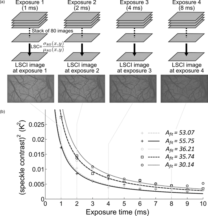 2.1.TheoryLSCI is based on calculating the speckle contrast K, defined as the ratio of standard deviation of the pixel intensity to the average intensity of the pixel. K can be calculated using two different schemes. The spatial scheme is the more widely used scheme1, 20 and involves calculation of speckle contrast K in a (n×n)-pixel window that slides within the acquired speckle image. The temporal scheme involves calculation of speckle contrast of every pixel calculated across a stack of m frames, sequentially in time. The temporal scheme is preferred when spatial resolution is paramount, and is the scheme employed in this study.13 The camera sensor integrates photons received over the exposure time for each image acquisition. Because LSCI captures motion, each exposure time is sensitive to a finite range of velocities. For example, LSCI at an exposure time of 5 ms might not capture the low blood flows characteristic of small caliber vessels, with an adequate CNR. Increasing the exposure time to 10 ms will permit flow measurements in these microvessels. However, at such high exposure times, the intensity-velocity sensitivity of large caliber vessels will be compromised. It has been previously shown that signal-to-noise ratio is maximum at an exposure time of 5 ms in rat brains.18 The relation of speckle contrast K to exposure time T is described in literature as21, 22 Eq. 1[TeX:] \documentclass[12pt]{minimal}\begin{document}\begin{equation} K^2 = \frac{{\tau _{\rm c} }}{{2T}}\left\{ {2 - \frac{{\tau _{\rm c} }}{T}\left[ {1 - \exp \left({ - \frac{{2T}}{{\tau _{\rm c} }}} \right)} \right]} \right\}, \end{equation}\end{document}Note that Eq. 1 is an improvement over the classical speckle equation proposed by Fercher and Briers.23 Equation 1 assumes that the speed model of the scatterers follows Lorentzian statistics. As long at the speckle optics do not change,21 the blood velocity may be assumed to vary linearly with 1/τc,24 and Eq. 1 reduces to the form Eq. 2[TeX:] \documentclass[12pt]{minimal}\begin{document}\begin{equation} K^2 = \frac{1}{{2BvT}}\left\{ {2 - \frac{{[ {1 - \exp ({ - 2BvT})} ]}}{{BvT}}} \right\}, \end{equation}\end{document}Because recent work has suggested that the relationship between 1/τc and blood velocity may be nonlinear,25 v should be considered as an indicator of blood velocity, rather than a measure of absolute velocity itself. 2.2.Imaging Procedure: Equipment and SetupThe LSCI procedure has been described in detail in Ref. 13. Briefly, the animal to be imaged was immobilized on a rigid frame and illuminated with a red (632 nm) He–Ne gas laser (JDSU, California). A stack of 80 images at a fixed exposure time was sequentially acquired using a 12-bit–cooled CCD camera (Cooke Corp., Mississippi) mounted with a 60-mm, f/2.8 macro lens. The magnification was set to 1:1, and the aperture was set to an f-number of 4.0, set such that the speckle diameter was approximately twice our pixel size of 6.7 μm, which is optimal for photographing speckles.26 The 80 images were processed off-line to calculate the temporal speckle contrast (K) using the following equation: Eq. 3[TeX:] \documentclass[12pt]{minimal}\begin{document}\begin{equation} K(x,y) = \frac{{\sigma _{80} (x,y)}}{{\mu _{80} (x,y)}}, \end{equation}\end{document}2.3.Multiexposure Laser Speckle Contrast Imaging Processing SchemeFor each pixel (x, y), LSC values corresponding to seven different exposure times were obtained by imaging the rat brain and this acquired stack K(x, y, T) of meLSCI data was fitted with a curve of the form Eq. 4[TeX:] \documentclass[12pt]{minimal}\begin{document}\begin{equation} K_{{\rm fit}}^2 = \frac{1}{{2A_{{\rm fit}} T}}\left\{ {2 - \frac{{[ {1 - \exp ({ - 2A_{{\rm fit}} T})} ]}}{{A_{{\rm fit}} T}}} \right\}. \end{equation}\end{document}2.4.Experimental ProtocolWe acquired meLSCI data from two experimental models. The benefits of meLSCI for blood-flow estimation were demonstrated in vivo in the widely used rat brain vasculature model, and its utility for longitudinal in vivo imaging was shown in a mouse ear wound healing model. 2.4.1.In vivo imaging of rat brain vasculatureFive adult female Fischer F344 rats were anesthetized and prepared as described previously.13 LSCI was done through the thinned skull of the rat under red laser illumination by serial acquisition of 80 frames of raw laser speckle images at seven different exposure times ranging from 1 to 7 ms. Care was taken to not disturb the preparation during image acquisition. Each rat underwent meLSCI on five different days. On each day, the same ROI was imaged, but the skull was rethinned to maintain optical transparency. 2.4.2.In vivo imaging of mouse ear vasculatureWe used eight immunocompetent, hairless SKH1 mice for this study and imaged the external ear using meLSCI. The mouse ear is ∼300 μm thick, and the planar microvasculature can be clearly visualized in the absence of fur; thus, this model has been used in a number of wound healing studies.27, 28 The mice were anesthetized with an intraperitoneal injection of 0.15 ml of a stock solution containing a mixture of ketamine (50 mg/kg) and xylazine (5 mg/kg). The right ear of each mouse was injured by creating a 2-mm-diam, full-thickness excision wound using a biopsy punch. The wound was wiped using ethanol swabs to prevent infection. The wounded mouse ear was gently restrained between a glass slide (bottom) and a cover slip (top) separated by 300-μm spacers. A small fixed weight (50 mg) was added to restrain the ears without occluding any vessels to maintain a constant pressure on the ear over several days of imaging. The mice were returned to the animal facility after imaging was complete and brought back at three and five days after wounding for follow up meLSCI. The same procedure was followed on all days of imaging (i.e., mice were reanesthetized and the ears were restrained for imaging). 3.ResultsThe meLSCI processing scheme was implemented on the raw laser speckle images of both rat brain and mouse ear vasculature, and the resulting images were compared to LSCI images obtained at a single exposure time to compare their performance. 3.1.Refined Image of Rat Brain Microvasculature Using meLSCIA fit was extracted by curve fitting the meLSC values at every pixel within the field of view and plotted as a pseudocolor map. Figure 2a shows the resulting high-resolution meLSCI image of rat brain vasculature. Because curve fitting is done on LSCI images processed using temporal contrast calculation, spatial resolution and vessel distinguishability (i.e., conspicuity) was high as compared to the image obtained using curve fitting on spatially processed LSCI images, as shown in Fig. 2b. As described in the ensuing section, it was determined that A fit calculated using meLSCI provided a refinement in velocity estimation than when 1/τc values were determined from LSCI at a single exposure time. Figure 2 demonstrates the need for such refinement in estimates by plotting the variability in the estimate of 1/τc values across the seven exposure times. Figures 2c, 2d, 2e show a qualitative comparison between independently obtained LSCI images (1/τc values) calculated using temporal contrast processing scheme at exposure times of 1, 2, and 5 ms. Figure 2f shows the exposure time–dependent variability in these images. This variability was computed as follows: the standard deviation of the 1/τc value for each pixel across seven different exposure times was calculated, normalized by the mean 1/τc value for that pixel, and plotted as a pseudocolor image. As can be seen in Fig. 2f, this exposure time–dependent variability can be as high as 25% for vessel pixels. Images were also smoothed [Figs. 2g, 2h, 2i] using a moving average window to remove the effect of stray pixels on the variability estimates. Although variability decreased with smoothing, as seen in Fig. 2j, it can still be as high as 17% for vessel pixels and higher for background tissue. Equivalent smoothed and unsmoothed LSCI images with spatial contrast calculated at 1-, 2-, and 5-ms exposure times along with the associated variability maps are shown in Figs. 2k, 2l, 2m, 2n, 2o, 2p, 2q, 2r. These images suggest substantially inferior performance of the spatial technique compared to the temporal processing scheme. Fig. 2High-resolution image of rat brain vasculature using meLSCI technique: (a) A high-resolution plot of the parameter A fit obtained by curve fitting the temporal LSC values at multiple exposure times (T 1–7 = 1, 2, 3, 4, 5, 6, and 7 ms) calculated using Eq. 4 for every pixel within the field of view. (b) A plot of parameter A fit similarly obtained by curve fitting the spatial LSC values at T. Note the ability of meLSCI in resolving microvessel details when it uses the temporal processing scheme. (c–e) Comparative plots of 1/τc values calculated using Eq. 2 for every pixel within the box in (a) at exposure times of 1, 2, and 5 ms, respectively. (f) The variation in LSC values at every pixel when acquired at T 1–7 calculated as the ratio of standard deviation to mean of each pixel across T 1–7. Note that error in most vessels is ∼20%. (g–j) These images are similar to (c–f), except that temporal LSC images were smoothed (median filter with window size 5×5) to prevent any effect of minor motion on the error. The error shown in (j) reveals values smaller than in (f) but still significant (∼10%). (k–n) and (o–r) show images analogous to (c–f) and (g–j), generated from unsmoothed and smoothed spatial LSC images, respectively. Note that the errors in (n) and (r) are very high. 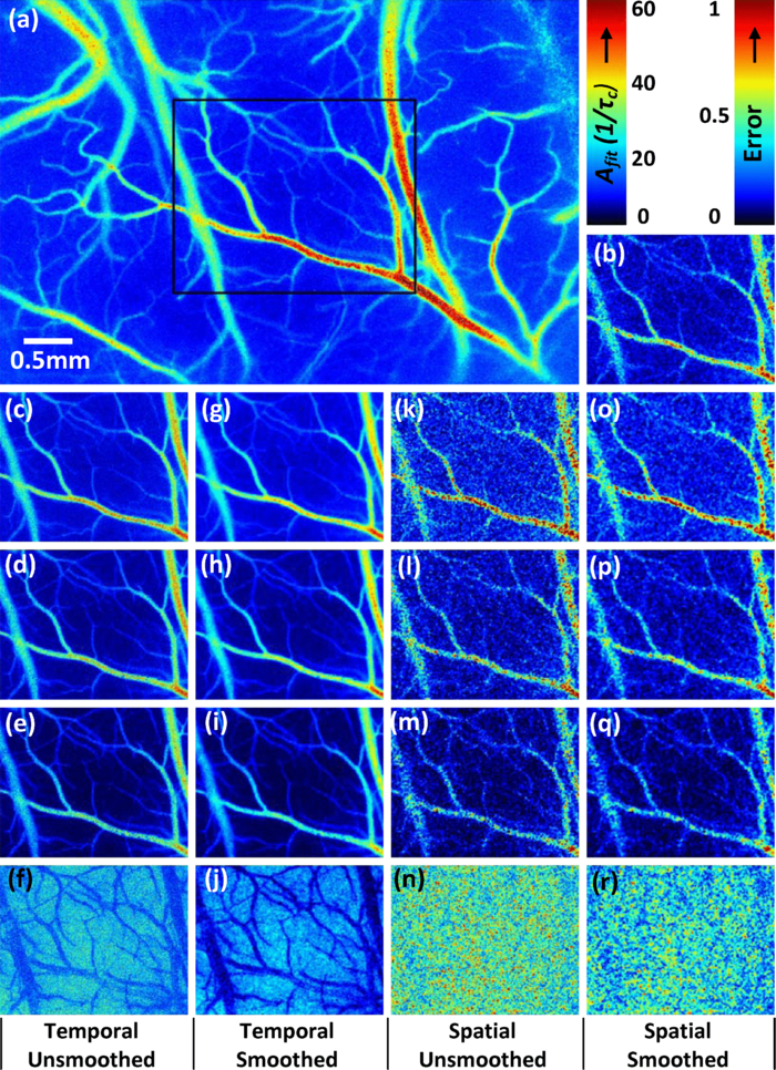 3.2.Evaluation of Multiexposure Laser Speckle Contrast Imaging Technique for Imaging Rat Brain VasculatureExperiments were performed as described above, and meLSCI images of brain surface were obtained from five rats over five imaging sessions (that is, over five days). These images were analyzed to obtain the following results. 3.2.1.Evaluation of curve fittingBoth spatial and temporal contrast values decrease with increasing exposure time and follow the exponential expression in Eq. 1. To analyze the accuracy of the curve fit, a set of 100 vessel pixels (x,y)1–100 were randomly chosen from the LSCI images of these rats (five rats×20 vessel pixels per rat) for statistical analysis. The coefficient of determination (R 2 value) was calculated for each pixel to determine the accuracy of the fit and found to be 0.92 ± 0.02 (mean ± standard error). In some images, our curve-fitting algorithm did not converge for some pixels. On investigation, these pixels were localized to image discrepancies such as intensity saturation from reflection from the occasional bubble in the sample preparation. 3.2.2.Multiexposure laser speckle contrast imaging produces flow estimates that are robust across multiple trialsmeLSCI produces estimates of blood flow that are robust across multiple trials compared to LSCI estimates of blood flow computed from a single exposure time. We showed that this improvement was attributable to the use of multiple exposure times rather than mere averaging of multiple images at a single exposure time. In each of 25 ROIs (five rats over five days), four different stacks of meLSC data were obtained and combined to obtain four meLSCI images. Each meLSCI image was generated by curve-fitting images obtained at four different exposure times (1, 2, 4, and 8 ms). The standard deviation of meLSC values across these four meLSCI images was calculated for every pixel and normalized to the mean meLSC value at the pixel. This normalized standard deviation (NSD) is an indicator of the variability in velocity estimates between images obtained as part of different trials, and thus a measure of robustness of velocity estimation over multiple imaging sessions. For comparison, four LSCI images were generated for each region and the 1/τc values averaged at exposure times of 1, 2, 4, and 8 ms. The NSD of 1/τc values was calculated across the four LSCI images and independently at each of the four exposure times. A comparison of the NSD, as obtained from meLSCI and LSCI schemes, is summarized in Table 1. Note that the NSD in meLSCI images is 0.238 ± 0.007 in vessel pixels and 0.247 ± 0.007 in background pixels, whereas the NSD in each of the averaged single-exposure-time LSCI images is higher (mean of 0.351 ± 0.007 in vessel pixels and 0.353 ± 0.006 in background pixels). This implies that meLSCI improves robustness of velocity estimation compared to simple averaging, by at least 30%. A two-tailed paired t-test between the meLSCI NSDs and each of the other LSCI NSDs demonstrated a significant (p < 0.0001) difference between the two methods, clearly demonstrating the superiority of meLSCI over averaging multiple images at any single exposure time. Fig. 5Use of meLSCI for imaging the microvascular environment during wound healing in a mouse ear injury model: (a–c) The top panel shows sequentially obtained meLSCI images of the mouse ear vasculature of the day of wounding, and three and five days after wounding. Note that the meLSCI scheme provides the contrast necessary to image the changes associated with neovascularization. (d–i) The middle panel shows high magnification views of the boxed region in (c), obtained using LSCI at single-exposure times and using meLSCI. 1/τc values have been depicted in pseudocolor. meLSCI can be clearly seen to have a higher contrast-to-noise ratio in proximal angiogenic regions by comparing (i) with (d–h). (j–n) The bottom panel shows equivalent high magnification views of the boxed region in (c), as they appear when the speckle contrast K is displayed in grayscale. Note that images (j–n) have been linearly and uniformly scaled for better print reproduction. Scale bar shown in (a) corresponds to 0.5 mm. 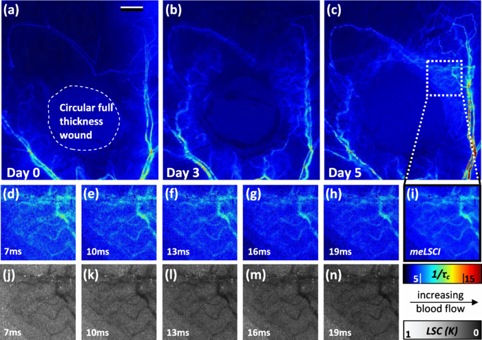 Table 1Comparison of NSD in meLSCI images to NSD in averaged LSCI images. The standard deviation of 1/τc values at every pixel across four LSCI images was calculated at each exposure time and normalized with the mean value to quantify the variability of 1/τc values across trials. The mean NSD values across all vessel and background pixels within an ROI was calculated and observed to be consistently lower in case of meLSCI processed images. The mean and standard deviation of these NSD values obtained from images of 25 ROIs (five rat brains×five days) are tabulated.
3.2.3.Use of seven different exposure times is optimal for multiexposure laser speckle contrast imaging processingIn this section, we explain why we used seven exposure times and how the robustness of meLSCI depends on the number of exposure times used. Toward this, meLSCI processing was done for all possible combinations of these exposure times taken two at a time, three at a time, and so on. In general, if the number of exposure times used in the meLSCI scheme is n T, then the number of images generated, N, in each case is N = 7 for n T = 1 (conventional LSCI), N = 21 for n T = 2, N = 35 for n T = 3, N = 35 for n T = 4, N = 21 for n T = 5, N = 7 for n T = 6, and N = 1 for n T = 7. We denote the image corresponding to n T = 7 as meLSCI7. Variation in flow estimates was calculated for each n T by calculating the NSD, as described previously, across N images generated by considering various combinations of exposure times. Vessel pixels were considered separately from background pixels, and a paired two-tailed t-test was performed to assess any differential dependence. As can be seen from Figs. 3a and 3b, the NSD of flow estimates decreased with increasing n T, and the p values indicated that there was not significant difference in this trend between vessel and background pixels. This suggests that the NSD is independent of the underlying blood flow. The NSD of the seven meLSCI images calculated from six exposure times was 0.075 ± 0.017, a significant improvement over the baseline NSD of 0.296 ± 0.067 in LSCI images obtained using only one of the seven different exposure times. We also analyzed how similar each image was to meLSCI7 by calculating the cross-correlation coefficient between each image and meLSCI7. The mean cross-correlation coefficient (averaged for the set of N images for each n T) increased with increasing n T, as shown in Fig. 3c. The maximum cross-correlation coefficient between meLSCI7 and each of the N images was seen to be considerably high for each n T, suggesting that at least one of the N images is very similar to the meLSCI7 image. In our experiment, exposure times of 1 and 2 ms seemed dominant as suggested by high cross-correlation coefficients of 0.92 between meLSCI7 and LSCI1ms and 0.84 between meLSCI7 and LSCI2ms. Also, the maximum cross-correlation corresponding to n T = 2 was as high as 0.99 when meLSCI7 was compared to an image generated by meLSCI processing of T = 1 ms and T = 2 ms. However, these dominant exposure times depend on the blood flow in those regions; that is, smaller low-flow vessels will be more accurately represented in images acquired at higher exposure times. The increase in the minimum cross-correlation with n T, as seen in Fig. 3c, demonstrates the robustness of the technique across larger flow regimes. The same trend also suggests convergence of the cross-correlation coefficient with increasing n T. Potentially, n T = 8 will further improve the performance of meLSCI but since the minimum cross-correlation between n T = 6 and n T = 7 was as high as 0.95, we deemed the use of seven exposure times to be accurate enough for our applications. Fig. 3Dependence of meLSCI images on the number of exposure times considered: (a,b) Dependence of the variation in flow estimates on the number of exposure times used in the meLSCI scheme. The mean and standard deviations have been calculated for data from five rats on five imaging days (25 cases in all). For each case, variation was calculated across all N images generated; that is, if number of exposure times used for meLSCI processing is denoted by n T, then for n T = 1, N = 7 (baseline LSCI); n T = 2, N = 21; n T = 3, N = 35; n T = 4, N = 35; n T = 5, N = 21; and for n T = 6, N = 7. Variation was calculated as normalized standard deviation of A fit (1/τc) values for every pixel across the N images. Results are shown differently for (a) vessel pixels and(b) background pixels though the variations in the two cases are very similar (p values of paired two-tailed t-tests between vessel and background pixels are indicated in (b). (c) The graph shows the cross-correlation between meLSCI images obtained at various values of n T with the image obtained at n(T) = 7. The cross-correlation was calculated for each of the N images generated at each value of n T and mean, maximum, and minimum cross-correlation across the N images was plotted for each n T. Note that while the maximum cross-correlation is very close to 1 even with n T = 2, suggesting two dominant exposure times, the minimum cross-correlation improves significantly suggesting that the robustness of meLSCI improves with increasing n T.  3.2.4.Multiexposure laser speckle contrast imaging improves microvessel distinguishabilitymeLSCI also improves the distinguishability of microvessels in addition to refining blood flow estimates. Figure 4a shows a region of the rat's brain, and flow estimates (1/τc and A fit values) along the indicated cross section, obtained at different exposure times, are shown in Fig. 4b. Note the low variability of the background pixel intensity in the meLSCI trace, as compared to traces at individual exposure times; and the high vessel distinguishability in the meLSCI, 3- and 5-ms traces as compared to the remaining traces. Statistical evaluation of the performance of meLSCI for microvessel distinguishability was done by comparing the CNR and distinguishable vessel length in meLSCI and LSCI images obtained from 3×3 mm regions of five rat brains. Note that the meLSCI images were obtained by curve-fitting data from ten exposure times (1–10 ms) and were compared to images generated by LSCI at exposure times of 1, 3, 5, 7, and 9 ms. Vessels that were distinguishable to the human eye were manually traced in each of the six images for every rat so as to paint all the vessel pixels black. Vessel length was counted by measuring the length along the centerlines in each of the manual traces (obtained by a binary skeletonization operation in MATLAB) as a metric for vessel distinguishability. As shown in Fig. 4c, we consistently observed an increase in distinguishable vessel length with increasing exposure time. meLSCI was often better at distinguishing vessels than single-exposure LSCI. Statistical analysis revealed that meLSCI resolved more microvessels, that is, more vessel length, than LSCI1ms by a factor of 1.53 ± 0.18 and LSCI5ms by a factor of 1.12 ± 0.08. As expected, this difference was attributable to the identification of microvessels, <20 μm diam (<3 pixels wide) as opposed to the larger vessels. CNR was calculated as follows: Eq. 5[TeX:] \documentclass[12pt]{minimal}\begin{document}\begin{equation} {\rm CNR} = \frac{{\mu _{{\rm vessel}} - \mu _{{\rm background}} }}{{\sigma _{{\rm background}} }}, \end{equation}\end{document}Fig. 4Distinguishability of microvessels using meLSCI technique: (a) An image of the rat brain brain vasculature obtained using meLSCI technique (using 10 exposure times, 1–10 ms). A fit values, indicative of blood velocity, are depicted in color. (b) Pixel intensities along the cross-section X-Y indicated in (a) as obtained by LSCI at various exposure times. Vessels are marked by numbers 1–9 and three significant background regions are marked by A, B, and C. Note the high background variation in the traces of 1–9 ms, as compared to the meLSCI trace. (c) The total length of distinguishable blood vessels was estimated in single-exposure LSCI and meLSCI images of 3×3 mm regions of five rat brains. The total vessel length is plotted relative to the vessel length extracted from the image at an exposure time of 1 ms. The distinguishability of vessels increased with exposure time and was highest for meLSCI images (plotted randomly at exposure time of 6 ms). (d,e) The CNRs of the images were analyzed and revealed that meLSCI resulted in a higher CNR than even the optimally recommended range of 3–5 ms for rat brain imaging. The increase in CNR can be primarily attributed to the low variability in the background signal. 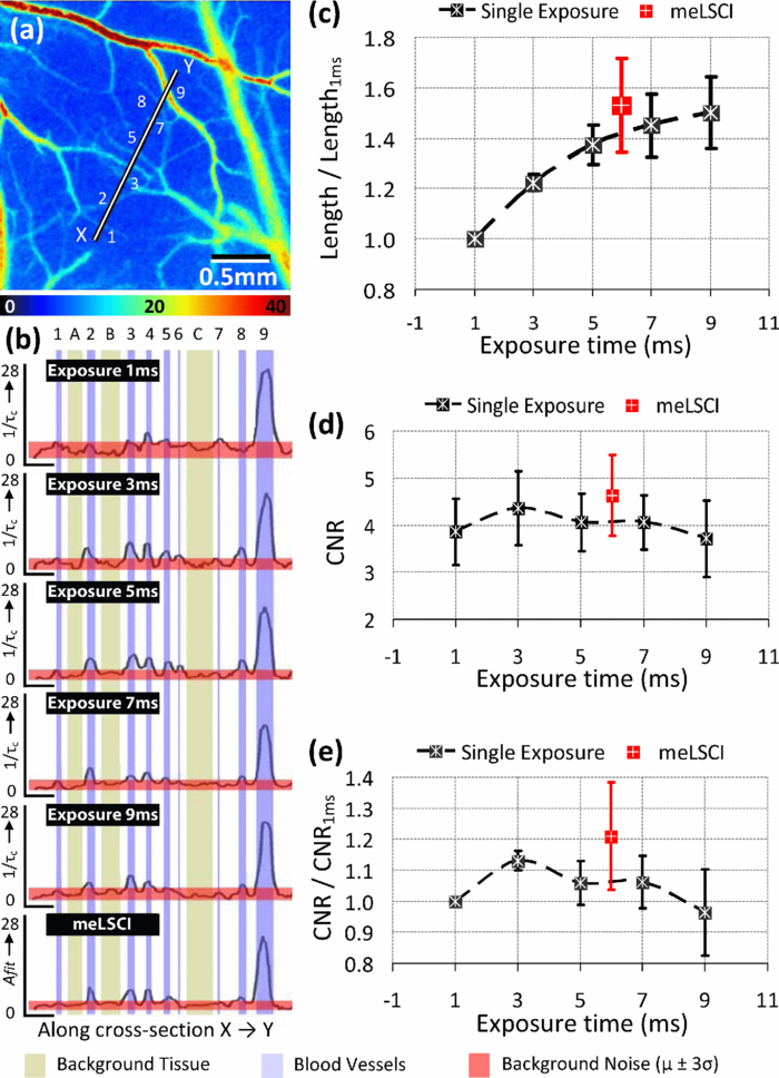 3.3.Imaging of Vascular Microenvironment during Wound Healing in Mouse Ear Using Multiexposure Laser Speckle Contrast ImagingThe advantage of meLSCI is that it can achieve better vessel distinguishability at a high CNR, while providing more robust blood-flow measurements. To demonstrate the advantages of meLSCI, we employed it to image the microvascular changes that accompany wound healing in an injured mouse ear model. Figure 5 shows sequential images of the region proximal to the wound, obtained on the day of wounding, three days after wounding, and five days after wounding. The wound causes an interruption in blood supply from two major vessels, causing the region downstream of the wound to receive limited blood flow through collateral circulation, as can be seen in the day 0 image. Extensive changes in vascularization and blood-flow redistribution were witnessed on days 3 and 5, and could be resolved with high CNR using meLSCI. Figures 5d, 5e, 5f, 5g, 5h, 5i illustrate high-magnification views of the neovascularized regions obtained at different exposure times. Figures 5j, 5k, 5l, 5m, 5n show comparative monochrome images of the same vascular microenvironment, as resolved traditionally through plotting the speckle contrast K, calculated using Eq. 3. It is apparent that meLSCI is able to resolve these microvessels with higher CNR than any of the contributing single-exposure-time images. CNR was calculated for this region, as described previously, and was found to be 2.28 as compared to a CNR of 1.80, which was best among all the LSCI images generated using single exposure times. For statistical analysis, we identified angiogenic regions in eight healing mice and compared the CNR values in these regions as imaged at single exposure times and using meLSCI. Table 2 lists the obtained mean CNR values, along with standard deviation, clearly indicating that meLSCI provides a 41% improvement in CNR in the region proximal to the wound. A two-tailed paired t-test demonstrated a significant difference (highest p = 0.0385) between the CNR values of meLSCI and every single-exposure-time LSCI image. This demonstrates the suitability of meLSCI for longitudinal monitoring of angiogenesis induced changes in the microvascular architecture and function. Table 2CNR for angiogenic regions in mouse ear model of wound healing. Angiogenic regions were identified in the region proximal to the wound in eight mice, and the CNR was determined for each of these identified regions, obtained at single-exposure times and using meLSCI. A two-tailed paired t-test was performed to determine whether the CNR values of meLSCI images were different from the CNR values of single-exposure-time LSCI images with statistical significance.
4.Discussion and ConclusionsIn this paper, we report a novel processing scheme, meLSCI, and demonstrate its use in vivo. meLSCI combines the high sensitivity of LSCI at low exposure times with higher vessel distinguishability possible with LSCI at high exposure times. In doing so, meLSCI produces blood-flow estimates that are more robust than estimates obtained from LSCI by simple averaging. We used pixelwise curve fitting to generate high spatial resolution images of vasculature in animal models of normal and pathological vasculature. We evaluated the robustness of the meLSCI technique in vivo and demonstrated that the variability in blood-flow estimates across multiple trials decreased by at least 30%. Vessel distinguishability was also at least as high as in the largest exposure time used, but the higher CNR of meLSCI images, especially in regions with high microvessel density, makes a strong case for its use in vascular imaging. Wound healing is accompanied by angiogenesis and is therefore an excellent model of vasculature undergoing remodeling. Imaging these microvascular changes is not trivial, especially due to the small size and low flow through angiogenic vessels. However, meLSCI was successfully able to capture the changes associated with this biological phenomenon. In the region proximal to the wound, meLSCI provided a 41% improvement in CNR over LSCI. This improvement in imaging specific regions was not accurately represented in our overall CNR analysis in rat brain vasculature, and hence, CNR in meLSCI images of rat brain seemed to improve only marginally. Thus, one could say that while the CNR in meLSCI images is at least as good as the best CNR of single-exposure LSCI images, meLSCI offered a clear advantage in imaging microvessels, <20 μm in diameter. meLSCI is a processing scheme, wherein LSCI images obtained at multiple exposures are combined to generate a parametrized image. However, the choice of exposure times as well as the number of exposure times that contribute to meLSCI is variable. It can be argued that meLSCI using only two exposure time (meLSCI2) with an accurate choice of both exposure times can produce fairly robust estimates that correlate well with meLSCI at seven exposure times (meLSCI7). However, choice of these two exposure times is not obvious and will depend heavily on the region of interest. For example, in the angiogenic regions where most of the vessels are small in size with low flow, meLSCI2 would be best at exposure times of 22 and 25 ms, but not in a region that has higher flow vessels. We used seven exposure times in most of our meLSCI estimations because the cross-correlation coefficient between meLSCI6 and meLSCI7 was 0.99, but more importantly, a minimum as high as 0.95. In our implementation of the meLSCI technique, we have assumed that the speed of scatterers contributing to the speckle signal follows Lorentzian statistics. As pointed out by Duncan and Kirkpatrick,21 a complete and precise treatment would require that both Lorentzian statistics (for random motion) and Gaussian statistics (for organized motion) be appropriately incorporated into the speckle equation [Eq. 2]. Our scheme, meLSCI, can be modified to use revised equations as well. We expect the results to be fairly model invariant, as suggested by our observation that replacing Eq. 2 by the widely used equation proposed by Fercher and Briers23 changed our results very marginally without affecting our conclusions. Similarly, recent work has also pointed out anomalies in the classically accepted linear relationship between blood velocity and parameter 1/τc. Ramirez-San-Juan present a detailed understanding of relationship between blood velocity and speckle statistics.25 The equations used in the meLSCI technique can continually be refined with the advent of more precise models. We have demonstrated that the combination of multiple images acquired at different exposure times improves the robustness of flow estimates and contrast-to-noise ratios in vivo. The robustness offered by the meLSCI technique should enable comparison of blood-flow estimates over multiple days of imaging with reduced errors due to imaging and sample preparation. However, it is not possible to demonstrate this in vivo because the physiological state of the animal cannot be eliminated as a source of variability. Despite our best standardization efforts, factors unrelated to imaging, such as degree of anesthesia or trauma, may cause the baseline blood flow to vary. We imaged the same rats on multiple days and observed a slight decrease in variability of the flow estimates across days using meLSCI. Although this difference was not statistically significant, ensuring an identical physiological state for each animal during imaging is challenging. A potential drawback of meLSCI is the additional time necessary for image acquisition. We used a processing scheme that acquired 80 frames at seven exposure times, or 560 frames at ∼10 fps (as supported by our camera). Thus, acquiring data required for generation of each meLSCI image took ∼60 s. Therefore, although meLSCI is suitable for longitudinal monitoring, it lacks the temporal resolution necessary for imaging rapid changes in blood flow. Also, rapid changes/fluctuations in blood flow will adversely affect the flow estimated by meLSCI because it inherently assumes that blood flow is constant during the acquisition of multiple-exposure data. The temporal resolution could be improved by increasing the image acquisition speed by imaging smaller regions or considering the use of fewer image frames for speckle contrast processing. However, in both these cases, the temporal resolution would come at the expense of spatial resolution. LSCI enjoys inherent advantages for vascular imaging in that blood flow can be imaged at a high spatial resolution without the need for an exogenous contrast agent. The meLSCI approach improves the contrast-to-noise ratio further and provides more reliable flow estimates, enabling sequential longitudinal monitoring of the vascular microenvironment. We foresee an application of meLSCI in understanding vascular reactivity at the “micro” level and elucidating the physiology of angiogenesis in a variety of disease states such as tumors or retinopathies. AcknowledgmentsThis work was supported jointly by National Institute of Aging Grant No. R01AG029681 and Department of Health and Human Services Grant No 1R43CA139983-01. The authors also thank Nicole Benoit, Peng Miao, and Dan Schlattman for their help with experimental preparation and Mohit Kumar Jolly for his help with preliminary in vitro experimentation. ReferencesA. K. Dunn, H. Bolay, M. A. Moskowitz, and
D. A. Boas,
“Dynamic imaging of cerebral blood flow using laser speckle,”
J. Cereb. Blood Flow Metab., 21
(3), 195
–201
(2001). https://doi.org/10.1097/00004647-200103000-00002 Google Scholar
J. S. Paul, A. R. Luft, E. Yew, and
F.-S. Sheu,
“Imaging the development of an ischemic core following photochemically induced cortical infarction in rats using laser speckle contrast analysis (LASCA),”
Neuroimage, 29
(1), 38
–45
(2006). https://doi.org/10.1016/j.neuroimage.2005.07.019 Google Scholar
V. Kalchenko, D. Preise, M. Bayewitch, I. Fine, K. Burd, and
A. Harmelin,
“In vivo dynamic light scattering microscopy of tumour blood vessels,”
J. Microsc., 228
(2), 118
–122
(2007). https://doi.org/10.1111/j.1365-2818.2007.01832.x Google Scholar
D. A. Boas and
A. K. Dunn,
“Laser speckle contrast imaging in biomedical optics,”
J. Biomed. Opt., 15
(1), 011109
(2010). https://doi.org/10.1117/1.3285504 Google Scholar
P. B. Jones, H. K. Shin, D. A. Boas, B. T. Hyman, M. A. Moskowitz, C. Ayata, and
A. K. Dunn,
“Simultaneous multispectral reflectance imaging and laser speckle flowmetry of cerebral blood flow and oxygen metabolism in focal cerebral ischemia,”
J. Biomed. Opt., 13
(4), 044007
(2008). https://doi.org/10.1117/1.2950312 Google Scholar
N. Li, X. Jia, K. Murari, R. Parlapalli, A. Rege, and
N. V. Thakor,
“High spatiotemporal resolution imaging of the neurovascular response to electrical stimulation of rat peripheral trigeminal nerve as revealed by in vivo temporal laser speckle contrast,”
J. Neurosci. Meth., 176
(2), 230
–236
(2009). https://doi.org/10.1016/j.jneumeth.2008.07.013 Google Scholar
P. Miao, N. Li, A. Rege, S. Tong and
N. Thakor,
“Model based reconstruction for simultaneously imaging cerebral blood flow and de-oxygen hemoglobin distribution,”
3236
–3293
(2009). https://doi.org/10.1109/IEMBS.2009.5333603 Google Scholar
M. Li, P. Miao, J. Yu, Y. Qiu, Y. Zhu, and
S. Tong,
“Influences of hypothermia on the cortical blood supply by laser speckle imaging,”
IEEE Trans. Neur. Sys. Rehab. Eng., 17
(2), 128
–134
(2009). https://doi.org/10.1109/TNSRE.2009.2012499 Google Scholar
J. Folkman,
“Tumor angiogenesis: therapeutic implications,”
N. Eng. J. Med., 285
(21), 1182
–1186
(1971). https://doi.org/10.1056/NEJM197108122850711 Google Scholar
P. Carmeliet and
R. K. Jain,
“Angiogenesis in cancer and other diseases,”
Nature, 407
(6801), 249
–257
(2000). https://doi.org/10.1038/35025220 Google Scholar
N. N. Nissen, P. J. Polverini, A. E. Koch, M. V. Volin, R. L. Gamelli, and
L. A. DiPietro,
“Vascular endothelial growth factor mediates angiogenic activity during the proliferative phase of wound healing,”
Am. J. Pathol., 152
(6), 1445
–1452
(1998). Google Scholar
A. P. Pathak, W. E. Hochfeld, S. L. Goodman, and
M. S. Pepper,
“Circulating and imaging markers for angiogenesis,”
Angiogenesis, 11
(4), 321
–335
(2008). https://doi.org/10.1007/s10456-008-9119-z Google Scholar
K. Murari, N. Li, A. Rege, X. Jia, A. All, and
N. V. Thakor,
“Contrast-enhanced imaging of cerebral vasculature with laser speckle,”
Appl. Opt., 46
(22), 5340
–5346
(2007). https://doi.org/10.1364/AO.46.005340 Google Scholar
C. J. Stewart, C. L. Gallant-Behm, K. Forrester, J. Tulip, D. A. Hart, and
R. C. Bray,
“Kinetics of blood flow during healing of excisional full-thickness skin wounds in pigs as monitored by laser speckle perfusion imaging,”
Skin Res. Tech., 12
(4), 247
–253
(2006). https://doi.org/10.1111/j.0909-752X.2006.00157.x Google Scholar
M. Le Thinh, J. S. Paul, H. Al-Nashash, A. Tan, A. R. Luft, F. S. Sheu, and
S. H. Ong,
“New insights into image processing of cortical blood flow monitors using laser speckle imaging,”
IEEE Trans. Med. Imag., 26
(6), 833
–842
(2007). https://doi.org/10.1109/TMI.2007.892643 Google Scholar
A. B. Parthasarathy, W. J. Tom, A. Gopal, X. Zhang, and
A. K. Dunn,
“Robust flow measurement with multi-exposure speckle imaging,”
Opt. Exp., 16
(3), 1975
–1989
(2008). https://doi.org/10.1364/OE.16.001975 Google Scholar
A. B. Parthasarathy, A. Ponticorvo, S. M. S. Kazmi, and
A. K. Dunn,
“Quantitative cerebral blood flow measurement through thinned skull with multi exposure speckle imaging,”
Frontiers in Optics, Optical Society of America(2009). Google Scholar
S. Yuan, A. Devor, D. A. Boas, and
A. K. Dunn,
“Determination of optimal exposure time for imaging of blood flow changes with laser speckle contrast imaging,”
Appl. Opt., 44
(10), 1823
–1830
(2005). https://doi.org/10.1364/AO.44.001823 Google Scholar
A. B. Parthasarathy, S. M. S. Kazmi, and
A. K. Dunn,
“Quantitative imaging of ischemic stroke through thinned skull in mice with multiexposure speckle imaging,”
Biomed. Opt. Exp., 1
(1), 246
–259
(2010). https://doi.org/10.1364/BOE.1.000246 Google Scholar
C. Ayata, A. K. Dunn, O. Y. Gursoy, Z. Huang, D. A. Boas, and
M. A. Moskowitz,
“Laser speckle flowmetry for the study of cerebrovascular physiology in normal and ischemic mouse cortex,”
J. Cereb. Blood Flow Metab., 24
(7), 744
–755
(2004). https://doi.org/10.1097/01.WCB.0000122745.72175.D5 Google Scholar
D. D. Duncan and
S. J. Kirkpatrick,
“Can laser speckle flowmetry be made a quantitative tool,”
J. Opt. Soc. Am. A, 25
(8), 2088
–2094
(2008). https://doi.org/10.1364/JOSAA.25.002088 Google Scholar
R. Bandyopadhyay, A. Gittings, S. Suh, P. Dixon, and
D. Durian,
“Speckle-visibility spectroscopy: a tool to study time-varying dynamics,”
Rev. Sci. Instrum., 76
(9), 0931101
–0931111
(2005). https://doi.org/10.1063/1.2037987 Google Scholar
A. R. Fercher and
J. D. Briers,
“Flow visualization by means of single-exposure speckle photography,”
Opt. Commun., 37
(5), 326
–330
(1981). https://doi.org/10.1016/0030-4018(81)90428-4 Google Scholar
M. Le Thinh, J. S. Paul, and
S. H. Ong,
“Laser speckle imaging for blood flow analysis,”
243
–271
(2009). https://doi.org/10.1007/978-1-4419-0811-7_11 Google Scholar
J. C. Ramirez-San-Juan, R. Ramos-García, I. Guizar-Iturbide, G. Martínez-Niconoff, and
B. Choi,
“Impact of velocity distribution assumption on simplified laser speckle imaging equation,”
Opt. Exp., 16
(5), 3197
–3203
(2008). https://doi.org/10.1364/OE.16.003197 Google Scholar
S. J. Kirkpatrick, D. D. Duncan, and
E. M. Wells-Gray,
“Detrimental effects of speckle-pixel size matching in laser speckle contrast imaging,”
Opt. Lett., 33
(24), 2886
–2888
(2008). https://doi.org/10.1364/OL.33.002886 Google Scholar
H. Sorg, T. Schulz, C. Krueger, and
B. Vollmar,
“Consequences of surgical stress on the kinetics of skin wound healing: partial hepatectomy delays and functionally alters dermal repair,”
Wound Repair Regen., 17
(3), 367
–377
(2009). https://doi.org/10.1111/j.1524-475X.2009.00490.x Google Scholar
J. H. Barker, D. Kjolseth, M. Kim, J. Frank, I. Bondar, E. Uhl, M. Kamler, K. Messmer, G. R. Tobin, and
L. J. Weiner,
“The hairless mouse ear: an in vivo model for studying wound neovascularization,”
Wound Repair Regen., 2
(2), 138
–143
(1994). https://doi.org/10.1046/j.1524-475X.1994.20208.x Google Scholar
|


