Tomographic x-ray–guided three-dimensional diffuse optical tomography of osteoarthritis in the finger joints

Zhen Yuan; Qizhi Zhang; Eric S. Sobel; Huabei Jiang

doi:10.1117/1.2965547

1 July 2008 Tomographic x-ray–guided three-dimensional diffuse optical tomography of osteoarthritis in the finger joints

Zhen Yuan, Qizhi Zhang, Eric S. Sobel, Huabei Jiang

Author Affiliations +

Journal of Biomedical Optics, Vol. 13, Issue 4, 044006 (July 2008). https://doi.org/10.1117/1.2965547

Abstract

We describe a multimodality imaging approach that combines x-ray tomosynthesis with near-infrared diffuse optical tomography (DOT) for high-resolution imaging of osteoarthritis in the finger joints. In this approach, we take advantage of high resolution x-ray imaging particularly of the bones and incorporate the fine structural maps obtained from x ray as a priori information into DOT reconstructions. To realize this multi-modality approach, we constructed a hybrid imaging platform that integrated a C-arm–based x-ray tomosynthetic system with a multichannel optic-fiber–based DOT system. We also implemented improved hybrid regularization-based reconstruction algorithms that have shown to be especially effective for high-resolution modality-guided DOT. Initial evaluation of our x-ray–guided DOT reconstruction approach in the finger joints shows that spatial resolution of DOT can be enhanced dramatically when the three-dimensional geometry of bones is known a priori. In particular, the improved quantitative capability of imaging absorption and scattering coefficients of the joint tissues allows for more accurate diagnosis of osteoarthritis over x-ray radiography or DOT alone.

1. Introduction

Osteoarthritis (OA) is the most common arthritic condition worldwide and is estimated to affect nearly 60 million Americans. Although a number of factors contribute to its development, including obesity, trauma, and genetic predisposition, the hallmark of OA is progressive damage to articular cartilage.¹ Classically, OA is most often found in the large weight-bearing joints of the lower extremities, particularly the knees and hips. However, there is also a subset of individuals with a predilection for developing OA of the hands and a more generalized form of OA.² Interestingly, it is the distal and proximal interphalangeal joints that are most often affected and culminate in the development of Heberden’s (distal) and Bouchard’s (proximal) nodes. To diagnose cartilage abnormalities and alterations in composition of synovial fluid in joints affected by OA, a variety of imaging methods have been developed and tested, such as radiography (x ray), ultrasound, computed tomography, and magnetic resonance imaging (MRI).^{3, 4, 5, 6, 7}

Of all the existing imaging modalities, x-ray radiography is the most widely accepted method for diagnosis of bone- and joint-related diseases, largely due to its high resolution $(\sim 0.1 mm)$ , its ease of use, and low cost. Although x ray has extremely high resolution in differentiating bones from soft tissues, it cannot distinguish well between soft tissues of similar densities, as the imaging contrast between different soft tissues is very low. For example, although plain radiographs are able to visualize joint space narrowing and osteophyte formation, they are insensitive to changes in cartilage and fluid and therefore incapable of capturing the primary features of the early stages of OA.⁸

Due to its numerous advantages of low cost, portability, and nonionizing radiation,⁹ near-infrared diffuse optical tomography (DOT) is emerging as a potential tool for imaging bones and joint tissues.^{10, 11, 12} In particular, DOT offers unparallel opportunity to access the molecular and cellular signatures that are contained in the absorption and scattering spectra of joint tissues.¹³ In a recent pilot clinical study, we have shown that the optical contrast between OA and normal joints is high,¹⁴ suggesting that DOT has the potential for detecting early OA joints in the hands. Although DOT appears to be especially suited for imaging of the finger joints because of the high signal-to-noise ratio associated with the small volume, the spatial resolution is relatively low due to the multiscattering events that occur along each photon path. Moreover, DOT reconstructions involve a typical ill-posed inverse problem with quite a few unknowns and limited numbers of measurements, which may further reduce the resolution.

Thus it is now clear that DOT can provide high-contrast joint tissue imaging with low resolution, but x ray can offer high-resolution joint structure with low contrast in soft tissues. To take advantage of the complementary information from these two kinds of imaging methods, we present a multimodality approach that combines x-ray and optical imaging for early diagnosis of OA in the finger joints. The basic idea of this multimodality approach is to incorporate the high-resolution x-ray images of joint tissues into the DOT reconstruction so that both the resolution and accuracy of optical image reconstruction are enhanced. In this study, a three-dimensional (3D) tomosynthetic x-ray method is used to coregister with the 3D DOT reconstruction of joint tissues. Even though an x-ray/DOT system will be more expensive than an x-ray system alone, it is certainly more economical than a MRI or ultrasound system.

In the remainder of this paper, we first describe our hybrid x-ray tomosynthesis and DOT system. We then present the finite element image reconstruction algorithms that are necessary for x-ray–guided optical image reconstruction. The integrated functioning of the hybrid imaging system and reconstruction algorithms are tested and evaluated through four typical clinical cases (two OA patients and two healthy volunteers). We discuss in detail the radiographic appearance of the four cases based on the qualitative optical images and quantitative optical properties as well as the thickness of the joint tissues (cartilage and fluid) in the distal interphalangeal (DIP) finger joint. Finally, the findings from the x-ray–guided optical images are compared with those from DOT or x-ray alone.

2. Experimental Materials and Methods

2.1.

Hybrid Imaging System

The hybrid x-ray/DOT imaging system integrates a modified mini C-arm x-ray system with a homemade $64 \times 64$ -channel photodiodes-based DOT system [see Fig. 1a ]. The DOT system has been described in detail previously.^{14, 15} Briefly, it consists of laser modules, a hybrid light delivery subsystem, a fiber optics/tissue interface, a data acquisition module, and light detection modules. A total of eight laser modules in the near-infrared region are available (the module at wavelength $853 nm$ was used in this study). An efficient and low-cost hybrid subsystem that comprises a $1 \times 8$ optical switch and a motorized rotator is used to deliver laser light to the excitation points along the fiber optics/tissue interface [the insert in Fig. 1a]. A total of 64 low-noise integrated silicon-photodiodes coupled with programmable circuit boards are used for parallel signal acquisitions. The entire LABVIEW-controlled data acquisition ( $64 \times 64$ channels) at one wavelength can be completed in $\sim 5 \min$ . The laser power used was $70 mW$ at $853 nm$ , giving a signal-to-noise ratio of $22 dB$ , and the illumination time was $2 to 3 s$ for each source location depending on the data acquisition time used for the 64 detectors. The core diameter of the source and detector optical fiber bundles was 1.0 and $2.0 mm$ , respectively.

Fig. 1

(a) Photograph of the integrated hybrid x-ray/DOT system. The insert is a close-view photograph of the finger/fiber optics/x-ray interface. (b) Schematic of the interface. Note that both the Plexiglass container and finger tip holder can be translated horizontally for separate DOT and x-ray data acquisition.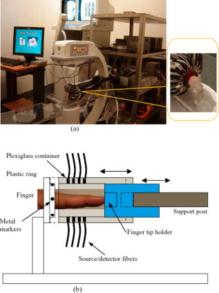

The tomosynthetic imaging is realized through a modified GE mini C-arm x-ray system (MiniView 6800, General Electric OEC, Salt Lake City, Utah). By mounting the C-arm on a personal computer–controlled rotator, x-ray projections can be obtained at any angle between 0 and $360 \deg$ with an accuracy of $0.01 \deg$ . In this study, the exposure dose applied to the target finger was lower than $10 mrad$ per projection with an exposure time of $2 s$ . The finger was typically placed $90 mm$ above the x-ray detector array, and while the distance between the x-ray tube and detector was $450 mm$ . Therefore, the actual size of the joint could be calculated by applying a factor of $4 ∕ 5$ .

The cylindrical fiber optics–tissue interface is composed of 64 source and 64 detector fiber bundles that are positioned in 4 layers along the surface of a Plexiglass container and cover a volume of $15 \times 30 mm$ . In each layer, 16 source and 16 detector fiber bundles are alternatively arranged. Light intensities were collected at 64 detector positions for each source location and a full set of $64 \times 64$ $(source \times detector)$ data was used for image reconstruction. The space between the finger and the wall of the Plexiglass container was filled with tissuelike phantom materials as coupling media consisting of distilled water, agar powder, Indian ink, and Intralipid, giving an absorption coefficient of $0.015 {mm}^{- 1}$ and a reduced scattering coefficient of $1.0 {mm}^{- 1}$ at $853 nm$ , which were optimized in our previous work.¹⁵ The relationships between the optical properties and the concentration of Indian ink and Intralipid were obtained through standard diffuse optical spectroscopic measurements using semi-infinite geometries.

In the hybrid imaging of joint tissues, the x-ray imaging is performed immediately after the DOT data acquisition. To eliminate the artifacts in the x-ray projections possibly caused by the optical interface, we have used a coaxial post to support the optical interface such that the interface can be translated along the post [see the insert in Fig. 1a and the schematic of the interface shown in Fig. 1b]. During an exam, the subject first places the finger into the Plexiglass container through a plastic ring while the distal end of the finger rests against a finger tip holder installed at the end of the coaxial post. Then the optical interface is slid to be in contact with the plastic ring structure that is used to lock the position of the optical interface. Immediately after the DOT imaging, the optical interface is slid back for x-ray exposure while the finger stays at the same position. Four small metal spheres ( $1 mm$ in diameter) are embedded along the surface of the plastic ring as fiducial markers for accurate coregistration of the x-ray and optical imaging.

2.2.

Image Reconstruction Algorithms

2.2.1.

X-ray image reconstruction

Tomographic x-ray images are reconstructed from two-dimensional projections using an improved shift-and-add algorithm we developed previously.¹⁶ In this algorithm, we first segment or normalize the projection images and then apply the shift-and-add algorithm (commonly used in digital tomosynthesis) on the segmented projection images at multiple angles, which results in accurate reconstruction of the 3D structures of joints. The method has been tested and evaluated using extensive phantom experiments.¹⁷ In this study, 16 projections were used and the resulting 3D x-ray images were displayed using commercial software called AMIRA (Visual Imaging, Carlsbad, California).

2.2.2.

X-ray–guided optical image reconstruction

Even though several methods are available in the area of a priori structural-guided DOT reconstruction, ^{18, 19, 20, 21, 22, 23, 24, 25, 26, 27, 28, 29, 30, 31, 32} regularization-based schemes appear to be the most effective as they can flexibly handle the problems associated with inaccurate domain segmentation that are required for a priori structural-guided DOT reconstruction. Several regularization-based schemes have been developed for MR- or x-ray–guided DOT reconstruction. ^{19, 20, 21, 22, 23, 24, 25, 26} However, most of these schemes do not appear to be able to handle the cases where MR or x ray is insensitive to the target tissues or lesions, resulting in inaccurate DOT reconstruction. In the area of joint imaging, for example, x ray is not able to detect the cartilage and fluids as well as their changes in the finger joints, although the changes associated with the cartilage and fluids can be easily captured by low-resolution DOT alone.¹⁴ In addition, the existing regularization schemes strongly depend on the choice of the initial optical property values and different initial guesses need to be specified for different tissue types. To overcome these limitations, we propose a modified Tikhonov or hybrid regularization technique for x-ray–guided DOT reconstruction.^{33, 34}

The conventional Tikhonov regularization for DOT sets up a weighted term as well as a penalty term to minimize the squared differences between computed and measured photon density values as follows:^{31, 35}

Eq. 1

\min_{χ} : {{‖ Φ^{c} - Φ^{o} ‖}^{2} + λ {‖ L δ χ ‖}^{2} = {{‖ Φ^{c} - Φ^{o} ‖}^{2} + λ {‖ L (χ - χ^{0}) ‖}^{2} .

The resulting updating equation based on Newton iterative method can be expressed as

Eq. 2

Δ χ = {(J^{T} J + λ L^{T} L)}^{- 1} [J^{T} (Φ^{o} - Φ^{c}) - λ L^{T} L χ],

in which

Φ^{o} = {(Φ_{1}^{o}, Φ_{2}^{o}, \dots, Φ_{M}^{o})}^{T}

and

Φ^{c} = {(Φ_{1}^{c}, Φ_{2}^{c}, \dots, Φ_{M}^{c})}^{T}

, where

Φ_{i}^{o}

and

Φ_{i}^{c}

are observed and computed photon densities for

i = 1, 2 \dots, M

boundary locations;

λ

is the Levenberg-Marquardt regularization parameter;

L

is the regularization matrix or filter matrix;

χ

expresses

μ_{a}

and

D

, where

μ_{a}

is the absorption coefficient and

D

is the diffusion coefficient, which can be written as

D = 1 ∕ [3 (μ_{a} + μ_{s}^{'})]

, where

μ_{s}^{'}

is the reduced scattering coefficient;

Δ χ = {(Δ D_{1}, Δ D_{2}, \dots, Δ D_{n}, Δ μ_{a, 1}, Δ μ_{a, 2}, \dots, Δ μ_{a, N})}^{T}

, and

Δ χ

is the updating vector for the optical properties; and

J

is the Jacobian matrix formed by

\partial Φ ∕ \partial χ

at the boundary measurement sites.

It should be noted the last term in Eq. 2 is not routinely used in the reconstruction and including the term would reduce the sharpness of known edges given a homogeneous initial guess. So we obtain the following updating equation when $λ = 1$ ,

Eq. 3

Δ χ = {(J^{T} J + L^{T} L)}^{- 1} [J^{T} (Φ^{o} - Φ^{c})] .

The most often used regularization matrix in DOT ise the identity matrix,³⁶ in which $L$ is a diagonal matrix and the prior information can be incorporated into the iterative process by using the spatially variant regularization parameter $λ$ .^{19, 23, 24} Other regularization algorithms include a subspace regularization scheme³⁵ or a total-variation minimization scheme,^{37, 38} where $L$ generated from MR or x-ray prior spatial information is a Gauss filter matrix,³⁵ or a Helmholtz³⁹ or Laplacian-type filter matrix.³¹ In this study, a Laplacian-type filter matrix $L$ was used, and its elements, $L_{i j}$ , were constructed according to the associated visible region or tissue-type x-ray-derived priors as follows:

Eq. 4

L_{i j} = {\begin{matrix} 1 & when i = j \\ - 1 ∕ n n & when i, j \subset one region \\ 0 & when i, j \subset different region \end{matrix},

where

N N

is the node number within a tissue type.

Instead of imposing constraints on the magnitude of the solution or on its derivative as in Tikhonov regularization, the developed regularization method minimizes the difference between the desired solution and its approximate x-ray or MR estimate, as well as the residual error in the least square sense. Hence in hybrid regularization-based nonlinear reconstruction algorithm, the objective function becomes

Eq. 5

\min : Ω = {‖ Φ^{c} - Φ^{o} ‖}^{2} + β [{‖ Φ^{c} - Φ^{0} ‖}^{2} + λ {‖ L (χ - χ^{0}) ‖}^{2}],

where

β

is the hybrid regularization parameter. By minimizing

Ω

with respect to

χ

(i.e.,

\partial Ω ∕ \partial χ = 0

) and considering Eq. 3, we obtain the following updating equation for the hybrid regularization:

Eq. 6

Δ χ = {(J^{T} J + β J^{T} J + λ^{'} I + β L^{T} L)}^{- 1} [J^{T} (Φ^{o} - Φ^{c})] .

If we specify the regularization parameter

β = 1

, Eq. 6 is simplified as,^{34, 40}

Eq. 7

Δ χ = {(J^{T} J + J^{T} J + λ^{'} I + L^{T} L)}^{- 1} [J^{T} (Φ^{o} - Φ^{c})],

in which

λ^{'}

is the Levenberg-Marquardt regularization parameter. It is noted from Eq. 7 that hybrid regularization is actually a regularization scheme that combines both Levenberg-Marquardt and Tikhonov regularization.^{34, 40} We have found that when

λ^{'} = (Φ^{o} - Φ^{c}) \times trace [J^{T} J]

, the reconstruction algorithm generates best results for x-ray–guided DOT reconstruction. Because joint tissues are highly heterogeneous, we have previously shown that a modified Newton method with excellent convergent property is required.^{14, 41} Thus the final updating equation for the developed scheme is modified as follows:

Eq. 8

χ_{new} = χ_{old} + ζ Δ χ (0 < ζ ⩽ 1),

where

ζ

is computed from a backtracking line search.⁴¹ Thus the realization of the excellent convergence algorithm is quite straightforward: the algorithm starts with a full Newton step (i.e.,

ζ = 1

) if the updated

χ

are close enough to the final solution, a quadratic convergence is obtained; if not, the backtracking line search will provide a smaller value of

ζ

along the Newton direction; the reconstruction process continues until a quadratic convergence is achieved.⁴¹

3. In Vivo Results

We present detailed studies on two healthy volunteers and two OA patients using the integrated hybrid system and x-ray–guided DOT reconstruction algorithm (extensive phantom evaluations were performed prior to the in vivo experiments that will be published elsewhere^{34, 42}). All the diseased joints were examined by a physician and showed clear signs of OA. The particular signs of OA joint were breakdown of joint cartilage; pain in a joint during or after use, or after a period of inactivity; discomfort in a joint before or during a change in the weather; swelling and stiffness in a joint, particularly after using it; bony lumps on the middle or end joints of fingers or the base of thumb; loss of joint flexibility; joint space narrowing, and so on.

Image reconstruction of each DIP joint with the optical coupling phantom/media, giving a cylindrical imaging volume of $30 (diameter) \times 20 (height) mm$ , was performed with a finite element mesh of 2 509 nodes and 10 752 tetrahedral elements. The 3D x-ray images of the joint allowed us to approximate the imaging domain into two types of tissue volumes: bones and joint tissues (cartilage, fluid, and phantom). The known anatomy of the bones from the x ray made it possible to automatically localize the finite element nodes (in side or outside the bone zone), allowing the Jacobian and filter matrices to be constructed within the same tissue type. The initial optical properties used were $μ_{s}^{'} = 1.2 {mm}^{- 1}$ and $μ_{a} = 0.04 {mm}^{- 1}$ for the bones and $μ_{s}^{'} = 1.0 {mm}^{- 1}$ and $μ_{a} = 0.01 {mm}^{- 1}$ for the soft joint tissues (cartilage, synovial fluid, and other components in the joint space) and the phantom, respectively. The source strength $S$ and boundary conditions coefficient $α$ were optimized using a preprocessing method described previously.³⁶ The entire image reconstruction took about $4 h$ with 20 iterations on a $2 - GHz$ Pentium IV personal computer for each case using FORTRAN code, and the preprocessing for the optimization of the initial parameters were achieved using MATLAB with only $1 to 2 \min$ for each case.

We note that the initial value of reduced scattering coefficient used for the joint tissues is not just for the synovial fluid: it is an effective value for all the soft tissues in the joint cavity including synovial fluid, cartilage, and other components. Because DOT does not have high enough resolution to distinguish between these different soft tissues within the joint space, it is impossible for us to assign different initial scattering values to the different soft tissue types. Although we are aware that the synovial fluid itself has a smaller scattering coefficient than the effective value used in our work, the used value of $μ_{s}^{'} = 1.0 {mm}^{- 1}$ is actually the scattering coefficient of the surrounding coupling medium, which is clearly known a priori. Using this value, we have found that the reconstructed averaged scattering coefficients of the soft tissues in the joint space for the cases studied are acceptable, as the calculated full width at half maximum (FWHM) based on these recovered values is comparable to that from x ray. The initial guesses for the optical properties of bones were estimated from our previous DOT reconstructions of the joints¹⁴ as well as from the literature.⁴³

Because joint space narrowing is an important measure of the degree of OA, a FWHM method was used to calculate the thickness of joint tissues (cartilage and fluid). For the FWHM method, we first took 12 representative dorsal (6 $x - z$ slices) and coronal slices (6 $y - z$ slices) from the reconstructed 3D optical images for quantitative analysis, which included 2 central slices in the dorsal and coronal planes, respectively. The 12 slices chosen were different for each in vivo case. For instance, for OA patient 1, the 6 dorsal slices were taken from $y = - 2 to 2 mm$ , and the 6 coronal slices were taken from $x = - 3 to 1 mm$ . The distance between two adjacent slices was less than $1 mm$ . Although the central dorsal and coronal slices went from $- 15 to 15 mm$ , the width of the other four slices was smaller than that of the central ones.

For each slice of the optical image, we plotted five central lines for quantitative analysis of absorption and scattering properties using FWHM, as shown in Fig. 2 . We limited the five lines within the joint domain. These lines were not always vertical, and for some cases, we used lines that were tilted and parallel to the middle line of the bones. Each FWHM curve was divided into two parts: bones and joint tissues (cartilage and fluid). By using FWHM, we calculated the mean thickness of joint tissues (cartilage and fluid), and we also provided the averaged optical properties of the bone and joint tissues. The quantitative results for the scattering and absorption coefficients are given in Tables 1, 2 , respectively, where the joint spacing estimated from the high-resolution x-ray images are also provided for comparison. Finally, DOT images without x-ray guidance for a healthy and a disease case are presented for additional comparison.

Fig. 2

(a) A 3D schematic of the finger joint measurement configuration. (b) Schematic of two-dimensional longitudinal/sagittal slice along with the five lines used for quantitative analysis using FWHM. (c) Schematic representative distribution of optical absorption coefficient along line $A B$ .

Table 1

Reconstructed μs′ related parameters for four cases.

Case		JointTissues	Averaged μs′ (1∕mm)	Mean thickness(mm)		μsc′∕μsb′
Case		JointTissues	Averaged μs′ (1∕mm)	DOT	X rays	μsc′∕μsb′
OA	1	Bone	1.60	N/A	N/A	0.82
		Joint	1.31	0.7	0.8
	2	Bone	1.42	N/A	N/A	0.83
		Joint	1.18	0.8	0.8

Healthy	3	Bone	1.67	N/A	N/A	0.52
		Joint	0.87	1.9	1.8
	4	Bone	1.92	N/A	N/A	0.49
		Joint	0.94	1.7	1.5

Note: μsc′ and μsb′ are the average reduced scattering coefficients of joint tissues and bone, respectively.N/A: Not available.

Table 2

Reconstructed μa related parameters for four cases.

Case		JointTissues	Averaged μa (1∕mm)	Mean thickness(mm)		μac∕μab
Case		JointTissues	Averaged μa (1∕mm)	DOT	X rays	μac∕μab
OA	1	Bone	0.044	N/A	N/A	0.75
		Joint	0.033	0.7	0.8
	2	Bone	0.041	N/A	N/A	0.76
		Joint	0.031	0.9	0.8

Healthy	3	Bone	0.041	N/A	N/A	0.20
		Joint	0.008	1.9	1.8
	4	Bone	0.052	N/A	N/A	0.35
		Joint	0.018	1.7	1.5

Note: μac and μab are the average absorption coefficients of joint and bone, respectively.N/A: Not available.

It should be noted that because the x-ray images contain errors on bone geometries, the geometric a priori knowledge from the x ray was not imposed directly on the DOT reconstructions; instead, the a priori information was added as a “soft” constraint on the DOT reconstructions through the use of the Laplacian-type filter matrix, which was able to relax the smoothness constraints at the interface between different regions or tissues. Thus the FWHM reconstructed by the x-ray–guided DOT is not the same as that by the x-ray images and is certainly better than that by DOT alone.

3.1.

Case 1: OA Patient 1

This patient was a $50 - year$ -old female, who was first diagnosed with OA in both joints of the index finger about $10 years$ ago. Figures 3a and 3b plot the scattering slices (along both dorsal and coronal planes) of the recovered 3D image, and Figs. 3c and 3d display the reconstructed absorption slices for this patient using the x-ray–guided DOT algorithms. The optical images without the x-ray guidance are given in Figs. 3e and 3f and the 3D x-ray images are shown in Fig. 3g for comparison.

Fig. 3

Reconstructed images at selected dorsal/coronal planes for case 1: (a) scattering slices along coronal planes ( $x - z$ plane) with x-ray guidance; (b) scattering slices along dorsal planes ( $y - z$ plane) with x-ray guidance; (c) absorption slices along coronal planes with x-ray guidance; (d) absorption slices along dorsal planes with x-ray guidance; (e) selected scattering slices without x-ray guidance; (f) selected absorption slices without x-ray guidance; (g) tomgraphic x-ray image from two different views. The axes (left and bottom) indicate the spatial scale in millimeters, whereas the color scale gives the absorption or scattering coefficient in inverse millimeters. (Color online only.)

3.2.

Case 2: OA Patient 2

The second patient was also a $50 - year$ -old female, whose DIP joint developed OA about $4 years$ ago. Figures 4a, 4b, 4c, 4d present the recovered scattering and absorption slices (along both dorsal and coronal planes) of the 3D images for this patient with the x-ray–guided DOT algorithms. In Fig. 4, we also give the 3D x-ray images [Fig. 4e] of the joint.

Fig. 4

Reconstructed images at selected dorsal/coronal planes for case 2: (a) scattering slices along coronal planes with x-ray guidance; (b) scattering slices along dorsal planes with x-ray guidance; (c) absorption slices along coronal planes with x-ray guidance; (d) absorption slices along dorsal planes with x-ray guidance; (e) tomgraphic x-ray image from two different views. (Color online only.)

3.3.

Case 3: Healthy Volunteers

The ages of the healthy volunteers were 32 and 40. Figures 5a, 5b, 5c, 5d display the recovered scattering and absorption slices (along both dorsal and coronal planes for the $32 - year$ -old volunteer) for a representative healthy case using the x-ray–guided DOT algorithms, where the optical images without the x-ray guidance and the 3D x-ray images are also provided.

Fig. 5

Reconstructed images at selected dorsal/coronal planes for case 3: (a) scattering slices along coronal planes with x-ray guidance; (b) scattering slices along dorsal planes with x-ray guidance; (c) absorption slices along coronal planes with x-ray guidance; (d) absorption slices along dorsal planes with x-ray guidance; (e) selected scattering slices without x-ray guidance; (f) selected absorption slices without x-ray guidance; (g) tomgraphic x-ray image from two different views. (Color online only.)

4. Discussion

In our x-ray–guided DOT reconstruction algorithms, we employed a full regularization matrix, which allowed the geometry of different tissue types to be predetermined by x-ray images. As shown in Figs. 3a, 3b, 3c, 3d, 4a, 4b, 4c, 4d, 5a, 5b, 5c, 5d, when a subset of the x-ray prior knowledge of the joint structure was used in the DOT reconstruction, distinct boundaries separating different tissues were recovered clearly, indicating the significant improvement of DOT resolution because of the incorporation of prior x-ray structural information. These optical images show accurate delineation of the joint space and bone geometry, that is consistent with the x-ray findings [Figs. 3g, 4e, 5g]. Both the absorption and scattering images reconstructed without x-ray guidance [Figs. 3e and 3f for the healthy controller and 5e and 5f for the patient] show significantly overestimated thickness of the joint tissues as well as increased boundary artifacts.

From the absorption and scattering images shown in Figs. 3, 4, 5, we also note that the bones are clearly delineated (most red-colored regions) for both OA and normal joints. Although there is no clear boundary between the cartilage and fluid, the joint tissues/space are clearly identified. Here the joint-space narrowing seems apparent for both OA joints (Figs. 3 and 4) relative to the healthy joints (Fig. 5). Importantly, compared with the optical parameters of the bones, we observe a large drop in the strength of absorption and scattering properties within the healthy joint space tissues. However, relative to the optical properties of the bones, we see only a small drop for the OA joint space tissues. Interestingly, the difference in scattering and absorption coefficients of the joint tissues (cartilage and synovial fluid) between the OA and healthy controls seems more striking from the ratio of scattering or absorption property to that of the bones (Tables 1, 2). We see that the ratios for both diseased joints are significantly larger than that for normal joints. The differences in the ratio between the OA and normal joints estimated from the x-ray–guided DOT reconstruction are notably increased relative to that without x-ray guidance.¹⁴

Judging from the structural size parameters listed in Tables 1, 2, we find that the mean thickness of cartilage and fluid in the OA joints seems thinner than those of the healthy ones. For example, as displayed in Table 1, for cases 1 and 2, the mean thickness of the joints (cartilage and fluid) computed from the scattering property distributions is 0.7 and $0.8 mm$ , respectively, compared with 1.9 and $1.7 mm$ for cases 3 and 4, respectively. Moreover, from Table 2, the mean thickness of the joints (cartilage and fluid) calculated from the absorption property distributions is 0.7 and $0.9 mm$ , respectively, for cases 1 and 2, relative to 1.9 and $1.7 mm$ for cases 3 and 4, respectively. This observation is further confirmed by the mean thickness of the joints estimated from the x-ray images, as shown in Tables 1, 2. It is also noted the joint space narrowing for the OA joints observed from the x-ray–guided DOT reconstruction is consistent with the x-ray findings [Figs. 3g, 4e, 5g and Table 1].

We note from Tables 1, 2 that the error of the recovered structural parameters is less than 10% compared with the x-ray findings. This is a significant improvement compared with that (typically more than 25%) from the DOT reconstruction without x-ray guidance.¹⁴ It is also interesting to note from Figs. 3, 4, 5 that the distributions of both absorption and scattering coefficients in the joint space are highly heterogeneous for OA patients, whereas such distributions are quite homogeneous in general for the healthy joints. We can also see from Tables 1, 2 that the structural parameters as well as the mean optical properties computed from the absorption and scattering distributions are generaly consistent with each other.

It should also be pointed out that model errors exist when the diffusion approximation is used to handle the cases involving low scattering, small source/detector distance, or large variations of optical properties. Although a transport model can certainly reduce such errors, we have previously and very recently shown that the model errors do not appear to propagate much to the reconstruction.^{10, 42} For example, the simulation tests from both our group and other groups indicate model errors typically result in about 10% error in reconstruction for small volume ptoblems.^{42, 44} Interestingly, for phantom and clinical experiments, the reconstruction errors are less than 10%. In addition to the use of diffusion approximation in DOT, many groups have used it to obtain high-quality image reconstructions for fluorescence and bioluminescent tomography of small animals where model errors certainly exist.^{45, 46, 47, 48} This is understandable because the accuracy of an inverse solution depends on not only the accuracy of the forward model, but also the quality of the experimental data and the use of robust regularization techniques. More interestingly, model errors lead to even smaller errors in reconstruction when the x-ray a priori structural information is incorporated into DOT reconstruction. This is because a more accurate modeling of photon migration through medium can be achieved when anatomical segmentation information becomes available. The use of prior structural information also eliminates the need to look for spatial/anatomy information in the optical inversion, which ensures that optical property profiles are the only parameters that needed to be recovered.

In summary, we have developed an imaging platform that integrates x-ray tomosynthesis with DOT along with a hybrid regularization-based reconstruction algorithm for the assessment of OA in the finger joints. The image quality obtained from the hybrid system is significantly improved over that from DOT alone. Enhanced x-ray–guided reconstruction results show that the optical properties as well as the joint spacing between OA and healthy joints are clearly different, suggesting that both types of imaging parameters could be used to diagnose OA and monitor its progression.⁴⁹

Acknowledgment

This research was supported in part by the National Institutes of Health (Grant No. R01 AR048122).

References

1.

P. Sarzi-Puttini, M. A. Cimmino, R. Scarpa, R. Caporali, F. Parazzini, A. Zaninelli, F. Atzeni, and B. Canesi, “Osteoarthritis: an overview of the disease and its treatment strategies,” Semin Arthritis Rheum., 35 1 –10 (2005). 0049-0172 Google Scholar

2.

D. J. Hart and T. D. Spector, “Definition and epidemiology of osteoarthritis of the hand: a review,” Osteoarthritis Cartilage, 8 S2 –S7 (2000). 1063-4584 Google Scholar

3.

W. P. Chan, P. Lang, M. P. Stevens, K. Sack, S. Majumdar, D. W. Stoller, C. Basch, and H. K. Genant, “Osteoarthritis of the knee: comparison of radiology, CT, and MR imaging to assess extent and severity,” Am. J. Roentgenol., 157 799 –806 (1991). 0092-5381 Google Scholar

4.

S. L. Myers, K. Dines, D. A. Brandt, K. D. Brandt, and M. E. Albrecht, “Experimental assessment by high frequency ultrasound of articular cartilage thickness and osteoarthritic changes,” J. Rheumatol., 22 109 –116 (1995). 0315-162X Google Scholar

5.

J. A. Tyler, P. J. Watson, H. L. Herrod, M. Robson, and L. D. Hall, “Detection and monitoring of progressive cartilage degeneration of osteoarthritic cartilage by MRI,” Acta Orthop. Scand. Suppl., 266 130 –138 (1995). 0300-8827 Google Scholar

6.

M. Forman, R. Malamet, and D. Kaplan, “A survey of osteoarthritis of the knee in the elderly,” J. Rheumatol., 10 282 –287 (1983). 0315-162X Google Scholar

7.

C. G. Peterfy, “Scratching the surface. Articular cartilage disorders of the knee,” MRI Clin. N. Am., 8 409 –430 (2000). Google Scholar

8.

J. T. Sharp, “Assessment of radiographic abnormalities in rheumatoid arthritis: what have we accomplished and where should we go from here,” J. Rheumatol., 22 1787 –1791 (1995). 0315-162X Google Scholar

9.

A. Yodh and B. Chance, “Spectroscopy and imaging with diffusing light,” Phys. Today, 48 34 –40 (1995). 0031-9228 Google Scholar

10.

Y. Xu, N. Iftimia, H. B. Jiang, L. L. Key, and M. B. Bolster, “Three-dimensional diffuse optical tomography of bones and joints,” J. Biomed. Opt., 7 88 –92 (2002). https://doi.org/10.1117/1.1427336 1083-3668 Google Scholar

11.

A. H. Hielscher, A. D. Klose, A. K. Scheel, B. Moa-Anderson, M. Backhaus, U. Netz, and J. Beuthan, “Sagittal laser optical tomography for imaging of rheumatoid finger joints,” Phys. Med. Biol., 49 1147 –1163 (2004). https://doi.org/10.1088/0031-9155/49/7/005 0031-9155 Google Scholar

12.

A. Pifferi, A. Torricelli, P. Taroni, A. Bassi, E. Chikoidze, E. Giambattistelli, and R. Cubeddu, “Optical biopsy of bone tissue: a step toward the diagnosis of bone pathologies,” J. Biomed. Opt., 9 474 –480 (2004). https://doi.org/10.1117/1.1691029 1083-3668 Google Scholar

13.

J. M. Lasker, E. Dwyer, and A. H. Hielscher, “Optical tomographic imaging of vascular and metabolic reactivity in rheumatoid joints,” Proc. SPIE, 5693 406 –416 (2005). 0277-786X Google Scholar

14.

Z. Yuan, Q. Zhang, and H. B. Jiang, “3D diffuse optical tomography imaging of osteoarthritis: initial results in finger joints,” J. Biomed. Opt., 12 034001 (2007). https://doi.org/10.1117/1.2737420 1083-3668 Google Scholar

15.

Q. Zhang and H. Jiang, “Three-dimensional diffuse optical tomography of simulated hand joints with a

64 \times 64

-channel photodiodes-based optical system,” J. Opt. A, Pure Appl. Opt., 7 224 –231 (2005). https://doi.org/10.1088/1464-4258/7/5/003 1464-4258 Google Scholar

16.

S. Li and H. Jiang, “A practical method for three-dimensional reconstruction of joints using a C-arm system and shift-and-add algorithm,” Med. Phys., 32 1491 –1499 (2005). https://doi.org/10.1118/1.1915289 0094-2405 Google Scholar

17.

H. Lou, Q. Zhang, C. Gibson, S. Li, and H. Jiang, “Digital tomosynthesis of joints based on a C-arm system,” J. X-Ray Sci. Technol., 13 1 –8 (2005). 0895-3996 Google Scholar

18.

Q. Zhu, N. G. Chen, and S. H. Kurtzman, “Imaging tumor angiogenesis by use of combined near-infrared diffuse light and ultrasound,” Opt. Lett., 28 337 –339 (2003). https://doi.org/10.1364/OL.28.000337 0146-9592 Google Scholar

19.

G. Gulsen, O. Birgul, and O. Nalcioglu, “Hybrid OT and MR system,” Proc. SPIE, 4955 246 –252 (2003). 0277-786X Google Scholar

20.

V. Ntziachristors, A. G. Yodh, M. Schnal, and B. Chance, “Concurrent MRI and diffuse optical tomography of breast after indocyanine green enhancement,” Proc. Natl. Acad. Sci. U.S.A., 97 2767 –2772 (2000). https://doi.org/10.1073/pnas.040570597 0027-8424 Google Scholar

21.

B. Brooksby, H. Dehghani, B. Pogue, and K. D. Paulsen, “Near Infrared (NIR) tomography breast reconstruction with a prior structural information from MRI: algorithm development reconstruction heterogeneities,” IEEE J. Sel. Top. Quantum Electron., 9 199 –209 (2003). https://doi.org/10.1109/JSTQE.2003.813304 1077-260X Google Scholar

22.

R. L. Barbour, H. L. Graber, J. Chang, S. S. Barbour, P. C. Koo, and R. Aronson, “MRI-guided optical tomography: prospects and computation for a new imaging method,” IEEE Comput. Sci. Eng., 2 63 –77 (1995). https://doi.org/10.1109/99.476370 1070-9924 Google Scholar

23.

Q. Zhang, T. J. Brukilacchio, A. Li, J. Scott, T. Chaves, E. Hillman, T. Wu, M. Chorlton, E. Rafferty, R. H. Moore, D. B. Kopans, and D. A. Boas, “Coregistered tomography x-ray and optical breast imaging: initial results,” J. Biomed. Opt., 10 024033 (2005). https://doi.org/10.1117/1.1899183 1083-3668 Google Scholar

24.

A. Li, E. L. Miller, M. E. Kilmer, T. J. Brukilaccio, T. Chaves, J. Scott, Q. Zhang, T. Wu, M. Choriton, R. H. Moore, D. B. Kopans, and D. A. Boas, “Tomographic optical breast imaging guided by three-dimensional mammography,” J. Biomed. Opt., 42 5181 –5190 (2003). 1083-3668 Google Scholar

25.

S. D. Konecky, R. Wienery, R. Choe, A. Corlu, K. Lee, S. M. Srinivasy, J. R. Saffer, R. Freifeldery, J. S. Karpy, and A. G. Yodh, “Diffuse optical tomography and position emission tomography of human breast,” (2006). Google Scholar

26.

M. Guven, B. Yazici, X. Intes, and B. Chance, “Diffuse optical tomography with a priori anatomical information,” Phys. Med. Biol., 50 2837 –2858 (2005). https://doi.org/10.1088/0031-9155/50/12/008 0031-9155 Google Scholar

27.

J. P. Kaipio, V. Kolehmainen, M. Vauhkonen, and E. Somersalo, “Inverse problems with structural prior information,” Inverse Probl., 15 713 –729 (1999). https://doi.org/10.1088/0266-5611/15/3/306 0266-5611 Google Scholar

28.

V. Ntziachristos, A. G. Yodh, M. D. Schnall, and B. Chance, “MRI-guided diffuse optical spectroscopy of malignant and benign breast lesions,” Neoplasia, 4 347 –354 (2002). https://doi.org/10.1038/sj.neo.7900244 1522-8002 Google Scholar

29.

B. W. Pogue and K. D. Paulsen, “High-resolution near-infrared tomographic imaging simulations of the rat cranium by use of a priori magnetic resonance imaging structural information,” Opt. Lett., 23 1716 –1718 (1998). https://doi.org/10.1364/OL.23.001716 0146-9592 Google Scholar

30.

M. Schweiger and S. R. Arridge, “Optical tomographic reconstruction in a complex head model using a priori region boundary information,” Phys. Med. Biol., 44 2703 –2721 (1999). https://doi.org/10.1088/0031-9155/44/11/302 0031-9155 Google Scholar

31.

B. Brooksby S. Jiang, H. Dehghani, B. W. Pogue, and K. D. Pausen, “Combining near-infrared tomography and magnetic resonance imaging to study in vivo breast tissues: implementation of a Laplacian-type regularization to incorporate magnetic resonance structure,” J. Biomed. Opt., 10 011504 (2005). https://doi.org/10.1117/1.2098627 1083-3668 Google Scholar

32.

B. W. Pogue, T. O. McBride, J. O. Prewitt, U. L. Osterberg, and K. D. Paulsen, “Spatially variant regularization improves diffuse optical tomography,” Appl. Opt., 38 2950 –2961 (1996). https://doi.org/10.1364/AO.38.002950 0003-6935 Google Scholar

33.

S. Twomey, “On the numerical solution of Fredholm integral equations of the first kind by the inverse of the linear system produced by quadrature,” J. Assoc. Comput. Mach., 10 97 –101 (1963). https://doi.org/10.1145/321150.321157 0004-5411 Google Scholar

34.

Z. Yuan and H. Jiang, “X-ray guided DOT reconstruction algorithm based on Twomey regularization,” Google Scholar

35.

B. Andrea, W. R. B. Lionheart, and C. N. McLeod, “Generation of anisotropic-smoothness regularization filters for EIT,” IEEE Trans. Med. Imaging, 21 579 –587 (2002). https://doi.org/10.1109/TMI.2002.800611 0278-0062 Google Scholar

36.

N. Iftimia and H. Jiang, “Quantitative optical image reconstruction of turbid media by use of direct-current measurements,” Appl. Opt., 39 5256 –5261 (2000). https://doi.org/10.1364/AO.39.005256 0003-6935 Google Scholar

37.

A. H. Hielscher and S. Bartel, “Use of penalty terms in gradient-based iterative reconstruction schemes for optical tomography,” J. Biomed. Opt., 6 183 –192 (2001). https://doi.org/10.1117/1.1352753 1083-3668 Google Scholar

38.

K. D. Paulsen and Huabei Jiang, “Enhanced frequency-domain optical image reconstruction in tissues through total-variation minimization,” Appl. Opt., 35 3447 –3458 (1996). 0003-6935 Google Scholar

39.

P. K. Yalavarthy, C. M. Carpenter, S. Jiang, H. Dehghani, B. W. Pogue, and K. D. Paulsen, “Incorporation of MR structural information in diffuse optical tomography using Helmholtz type regularization,” (2006). Google Scholar

40.

Z. Liu, F. Kecman, and B. He, “Effects of fMRI-EEG mismathes in cortical current density estimation integrating fMRI and EEG: A simulation study,” Clin. Neurophysiol., 117 1610 –1622 (2006). 1388-2457 Google Scholar

41.

Z. Yuan and H. Jiang, “Image reconstruction schemes that combines modified Newton method and efficient initial guess estimate for optical tomography of finger joints,” Appl. Opt., 46 2757 –2768 (2007). https://doi.org/10.1364/AO.46.002757 0003-6935 Google Scholar

42.

Z. Yuan, Q. Zhang, and H. Jiang, “X-ray guided diffuse optical imaging of small volume tissues based on

p_{3}

approximated radiative transport equation,” Google Scholar

43.

P. Taroni, D. Comelli, A. Farina, and A. Pifferi, “Time-resolved diffuse optical spectroscopy of small tissues samples,” Opt. Express, 15 3301 –3311 (2007). https://doi.org/10.1364/OE.15.003301 1094-4087 Google Scholar

44.

K. Ren, G. Bal, and A. Hielscher, “Transport and diffusion-based optical tomography in small domains: a comparative study,” Appl. Opt., 46 6669 –6679 (2007). https://doi.org/10.1364/AO.46.006669 0003-6935 Google Scholar

45.

V. Ntziachristos, T. Jacks, R. Weissleder, J. Grimm, D. G. Kirsch, S. D. Windsor, C. F. Bender Kim, and P. M. Santiago, “Use of gene expression profiling to direct in vivo molecular imaging of lung cancer,” Proc. Natl. Acad. Sci. U.S.A., 102 14404 –14409 (2005). https://doi.org/10.1073/pnas.0503920102 0027-8424 Google Scholar

46.

A. K. Sahu, R. Roy, A. Joshi, and E. M. Sevick-Muraca, “Evaluation of anatomical structure and non-uniform distribution of imaging agent in near-infrared, fluorescence-enhanced optical tomography,” Opt. Express, 13 10182 –10199 (2005). https://doi.org/10.1364/OPEX.13.010182 1094-4087 Google Scholar

47.

L. Hervé, A. Koenig, A. Da Silva, M. Berger, J. Boutet, J. M. Dinten, P. Peltié, and P. Rizo, “Noncontact fluorescence diffuse optical tomography of heterogeneous media,” Appl. Opt., 46 4896 –4906 (2007). https://doi.org/10.1364/AO.46.004896 0003-6935 Google Scholar

48.

G. Wang, W. Cong, K. Durairaj, X. Qian, H. Shen, P. Sinn, E. Hoffman, G. McLennan, and M. Henry, “In vivo mouse studies with bioluminescence Tomography,” Opt. Express, 14 7801 –7809 (2006). https://doi.org/10.1364/OE.14.007801 1094-4087 Google Scholar

49.

E. Naredo, I. Moller, C. Moragues, J. J. de Agustin, A. K. Scheel, W. Grassi, E. de Miguel, M. Backhaus, “Interobserver reliability in musculoskeletal ultrasonography: results from a ‘Teach the Teachers’ rheumatologist,” Ann. Rheum. Dis., 65 14 –19 (2006). https://doi.org/10.1136/ard.2005.037382 0003-4967 Google Scholar

Citation Download Citation

Zhen Yuan, Qizhi Zhang, Eric S. Sobel, and Huabei Jiang "Tomographic x-ray–guided three-dimensional diffuse optical tomography of osteoarthritis in the finger joints," Journal of Biomedical Optics 13(4), 044006 (1 July 2008). https://doi.org/10.1117/1.2965547

Published: 1 July 2008

Access the abstract

JOURNAL ARTICLE
10 PAGES

DOWNLOAD PAPER SAVE TO MY LIBRARY

GET CITATION

CITATIONS

Cited by 55 scholarly publications.

Explore citations on Lens.org

RIGHTS & PERMISSIONS

Get copyright permission Get copyright permission on Copyright Marketplace

KEYWORDS

X-rays

X-ray imaging

Tissues

Scattering

Bone

Absorption

Reconstruction algorithms

1.

Introduction

2.

Experimental Materials and Methods

2.1.

Hybrid Imaging System

Fig. 1

2.2.

Image Reconstruction Algorithms

2.2.1.

X-ray image reconstruction

2.2.2.

X-ray–guided optical image reconstruction

Eq. 1

Eq. 2

Eq. 3

Eq. 4

Eq. 5

Eq. 6

Eq. 7

Eq. 8

3.

In Vivo Results

Fig. 2

Table 1

Table 2

3.1.

Case 1: OA Patient 1

Fig. 3

3.2.

Case 2: OA Patient 2

Fig. 4

3.3.

Case 3: Healthy Volunteers

Fig. 5

4.

Discussion

Acknowledgment

References

Show All Keywords

Keywords/Phrases

Search In:

Publication Years